LLM Systems 07: Pre-trained LLMs

0. Recap

• Sequence-to-sequence encoder-decoder framework for conditional generation, including Machine Translation
• Key components in Transformer
  • Positional Embedding (to distinguish tokens at different pos)
  • Multihead attention
  • Residual connection
  • Layer norm

1. Pretrained Encoder-Decoder LLM: T5

• Exploring the Limits of Transfer Learning with a Unified Text-to-Text Transformer
• arXiv 提交日期：23 Oct 2019；发表于 Journal of Machine Learning Research 2020
• 作者：其中 Noam Shazeer 也是 Transformer 论文作者
  

1.1 Model Architecture & Model Size

• 模型架构：标准 Encoder-Decoder Transformer
  • 解码方式 (Decoding)：Beam search（Beam width=4, Length penalty=0.6）
  • Length penalty=0.6：用于修正 Beam Search 对短序列的偏好。公式为 \(\frac{\log P}{|Y|^{0.6}}\)。0.6 是一个经验折中值，既避免了模型生成过短的残缺文本，又防止了生成过于冗长啰嗦的句子。
• 模型规模：
  • T5-base: 220M parameters (12 blocks, \(d_{ff} = 3072\), \(d_{kv} = 64\), 12-headed attention, \(d_{model} = 768\))
  • T5-3B: 24 blocks, \(d_{model} = 1024\), \(d_{kv} = 128\), \(d_{ff} = 16384\), 32-headed attention
  • T5-11B: 24 blocks, \(d_{model} = 1024\), \(d_{kv} = 128\), \(d_{ff} = 65536\), 128-headed attention

注意： 上述 3B/11B 模型，不满足 \(d_{kv} \times h = d_{model}\) （其中 \(h\) 表示 MHA heads 数量）。这是因为 T5 模型修改了 Q/K/V/O 的权重矩阵的维度，对 Q/K/V 进行了维度扩展，然后进行 Attention 计算。相关代码如下：

• https://github.com/huggingface/transformers/blob/main/src/transformers/models/t5/configuration_t5.py

  @auto_docstring(checkpoint="google-t5/t5-small")
  @strict
  class T5Config(PreTrainedConfig):
      r"""
      relative_attention_num_buckets (`int`, *optional*, defaults to 32):
          The number of buckets to use for each attention layer.
      relative_attention_max_distance (`int`, *optional*, defaults to 128):
          The maximum distance of the longer sequences for the bucket separation.
      feed_forward_proj (`string`, *optional*, defaults to `"relu"`):
          Type of feed forward layer to be used. Should be one of `"relu"` or `"gated-gelu"`. T5v1.1 uses the
          `"gated-gelu"` feed forward projection. Original T5 uses `"relu"`.
      """
  
      model_type = "t5"
      keys_to_ignore_at_inference = ["past_key_values"]
      attribute_map = {
          "hidden_size": "d_model",
          "num_attention_heads": "num_heads",
          "num_hidden_layers": "num_layers",
          "head_dim": "d_kv",
      }
  
      vocab_size: int = 32128
      d_model: int = 512
      # 单独初始化
      d_kv: int = 64
      d_ff: int = 2048
      num_layers: int = 6
      num_decoder_layers: int | None = None
      # 单独初始化
      num_heads: int = 8
      relative_attention_num_buckets: int = 32
      relative_attention_max_distance: int = 128
      dropout_rate: float | int = 0.1
      layer_norm_epsilon: float = 1e-6
      initializer_factor: float = 1.0
      feed_forward_proj: str = "relu"
      is_encoder_decoder: bool = True
      use_cache: bool = True
      pad_token_id: int | None = 0
      eos_token_id: int | list[int] | None = 1
      classifier_dropout: float | int = 0.0
      is_decoder: bool = False

• https://github.com/huggingface/transformers/blob/main/src/transformers/models/t5/modeling_t5.py

  class T5Attention(nn.Module):
      def __init__(
          self,
          config: T5Config,
          has_relative_attention_bias=False,
          layer_idx: int | None = None,
          is_causal: bool = False,
      ):
          super().__init__()
          self.config = config
          self.is_decoder = config.is_decoder
          self.is_causal = is_causal
          self.has_relative_attention_bias = has_relative_attention_bias
          self.relative_attention_num_buckets = config.relative_attention_num_buckets
          self.relative_attention_max_distance = config.relative_attention_max_distance
          self.d_model = config.d_model
          self.key_value_proj_dim = config.d_kv
          self.n_heads = config.num_heads
          self.dropout = config.dropout_rate
          # 注意这里 inner_dim 计算
          self.inner_dim = self.n_heads * self.key_value_proj_dim
          
          # 省略部分代码 ...
  
  		# QKVO 权重矩阵 shape
          self.q = nn.Linear(self.d_model, self.inner_dim, bias=False)
          self.k = nn.Linear(self.d_model, self.inner_dim, bias=False)
          self.v = nn.Linear(self.d_model, self.inner_dim, bias=False)
          self.o = nn.Linear(self.inner_dim, self.d_model, bias=False)
  
          # 省略部分代码 ...

1.2 Training

• 整体流程：Pre-training \(\rightarrow\) Multitask Finetuning
• Pre-training：
  • 数据集：C4 (Colossal Clean Crawled Corpus)，来自 Common Crawl 过滤出的英语语料库，规模 750GB。
  • 目标：Recover randomly corrupted spans（随机破坏 15% 的文本片段，Cloze-style，即：完形填空式预训练）。
  • 示例：Original: Thank you for inviting me to your party last week. -> Inputs: Thank you <X> me to your party <Y> week. -> Targets: <X> for inviting <Y> last <Z>
  • 哨兵 token (Sentinel Tokens)：T5 词表中额外的 100 个特殊 token（<extra_id_0> ~ <extra_id_99>，上述示例简写为 <X>, <Y>, <Z>）。在输入中充当被挖空片段的占位符；在目标输出中作为每个被挖空片段的前缀引导符，并在末尾额外加一个哨兵 token 作为 EOS 结束符。这种设计使得模型能够按顺序、精确地生成多个被破坏的连续片段。
  • 训练细节：Pre-train 0.5M steps；Batch size = 128 sequences (sequence length=512，packing multiple seqs 65k tokens per batch)；Result in 34B trained tokens。
• Supervised fine-tuning：
  • 语言理解/文本分类：GLUE / SuperGLUE
  • 摘要生成：CNN/Daily mail corpus
  • 问答：SQuAD
  • 机器翻译：WMT English to German, French, Romanian
• Multitask SFT with Task Instruction：
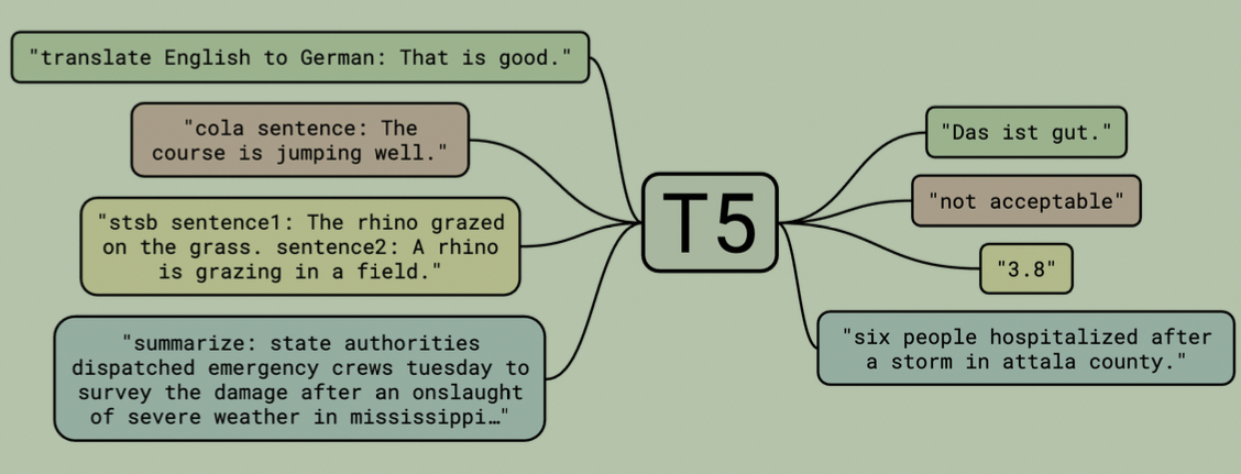
  • 核心思想：Unified format to put task instructions as natural language in the input，enables transfer to new tasks。
  • 将所有下游任务转为“前缀 + 输入文本 → 输出文本”的统一格式，混合所有任务数据一起微调。损失函数与预训练相同（Decoder 端交叉熵），使用 teacher forcing。模型通过任务前缀区分不同任务，实现一个模型处理多种 NLP 任务。
  • 输入输出示例：
  • 后续发展：With more instruction tuning \(\rightarrow\) T0, Flan-T5。
    • T5 的“多任务 SFT”依赖固定任务前缀；指令微调改用大量自然语言指令 → 输出数据，显著提升零样本 / 新任务泛化能力。
    • T0 （arXiv 提交日期：15 Oct 2021，ICLR 2022）：基于 T5，用 P3（多任务、多提示模板）做指令微调；T0-11B 在多个零样本 NLP 任务上超过 GPT-3 175B，参数量约小 16 倍，展示了指令微调对零样本泛化的显著提升。
    • Flan-T5（arXiv 提交日期：20 Oct 2022，Journal of Machine Learning Research 2024）：基于 T5，用更大更多样的 Flan 2022 指令集合 + CoT 训练，性能全面超越 T0/T5，下游微调收敛更快、效果更好。

T5 训练&推理流程：

┌─────────────────────────────────────────────────────────┐
│  训练阶段                                                │
│                                                         │
│  原文 ──span corruption──→ input (带哨兵) + label (带哨兵)│
│                                                         │
│  input  → Encoder → hidden_states                       │
│  label  → 右移 → Decoder + cross-attention → logits     │
│  logits vs label → Cross-Entropy Loss                   │
└─────────────────────────────────────────────────────────┘

┌─────────────────────────────────────────────────────────┐
│  推理阶段                                                │
│                                                         │
│  input → Encoder → hidden_states                        │
│  Decoder 从 <pad> 开始自回归生成                         │
│  每步：用已生成的 token 作为下一步输入                    │
│  Beam Search 保留 top-4 候选                             │
│  直到生成 EOS 或达到最大长度                              │
│  输出 token 序列 → 解码为文本                             │
└─────────────────────────────────────────────────────────┘

• 训练：input 和 label 是分离的。Encoder 编码被破坏的输入，Decoder 用 teacher forcing 接收右移的 label（即：pad 起始 token + label[:-1] 序列除了最后一个 token 输入，预测完整的 label），通过 cross-attention 关注 Encoder 输出，对所有位置并行计算交叉熵 loss。
• 推理：没有 label。Decoder 从起始 token 开始，自回归逐步生成，每步把已生成的 token 追加到输入中。使用 Beam Search（width=4, length penalty=0.6）保留最优候选，直到生成 EOS。
• 核心区别：训练时所有位置并行计算 loss；推理时必须串行逐步生成。

指令微调补充：

• 本质：用大量“自然语言指令 → 输出”数据训练，让模型学会遵循任意指令，提升零样本/新任务泛化。
• 数据格式：通常含 instruction、input（选填）、output。常用 Alpaca 格式：

  {"instruction": "任务描述", "input": "上下文（选填）", "output": "期望回答"}

  训练时填入固定模板：### Instruction: {instruction} ### Input: {input} ### Response: {output}，input 为空时省略 ### Input:。编码器输入为 instruction+input 拼接，解码器目标为 output。
• 损失函数：掩码下一词交叉熵，只计算 output 部分；instruction 和 input 部分不参与 loss。
• 训练：混合所有任务指令数据，按比例采样；T0 用 P3（多任务多模板），Flan-T5 用 Flan 2022 + CoT。
• 推理：自回归生成，面对未见指令直接生成输出（零样本）；也可给少量示例（少样本）。
• 与 T5 多任务微调区别：T5 用固定任务前缀，学执行特定任务；指令微调用自然语言指令，学遵循任意指令，泛化更强。
• 注意：指令微调存在适应性与泛化权衡，效果依赖指令数据质量、多样性和模板一致性。

2. Pretrained Decoder-Only LLMs: LLaMA

2.1 Model Architecture & Model Size

• LLaMA: Open and Efficient Foundation Language Models

• arXiv 提交日期：27 Feb 2023

• GitHub：https://github.com/meta-llama/llama

• 作者：
  Model Architecture

• Based on Transformer decoder-only, with a few improvements

• Pre-normalization（来自 GPT3）

• RMSNorm

• SwiGLU activation function（来自 PaLM: Swish-Gated Linear Unit）

• Rotary Embeddings（来自 RoFormer）

关键代码摘录：

# config
@dataclass
class ModelArgs:
    dim: int = 4096
    n_layers: int = 32
    n_heads: int = 32
    n_kv_heads: Optional[int] = None
    vocab_size: int = -1  # defined later by tokenizer
    multiple_of: int = 256  # make SwiGLU hidden layer size multiple of large power of 2
    ffn_dim_multiplier: Optional[float] = None
    norm_eps: float = 1e-5

    max_batch_size: int = 32
    max_seq_len: int = 2048


class FeedForward(nn.Module):
    def __init__(
        self,
        dim: int,
        hidden_dim: int,
        multiple_of: int,
        ffn_dim_multiplier: Optional[float],
    ):
        """
        Initialize the FeedForward module.

        Args:
            dim (int): Input dimension.
            hidden_dim (int): Hidden dimension of the feedforward layer.
            multiple_of (int): Value to ensure hidden dimension is a multiple of this value.
            ffn_dim_multiplier (float, optional): Custom multiplier for hidden dimension. Defaults to None.

        Attributes:
            w1 (ColumnParallelLinear): Linear transformation for the first layer.
            w2 (RowParallelLinear): Linear transformation for the second layer.
            w3 (ColumnParallelLinear): Linear transformation for the third layer.

        """
        super().__init__()
        hidden_dim = int(2 * hidden_dim / 3)
        # custom dim factor multiplier
        if ffn_dim_multiplier is not None:
            hidden_dim = int(ffn_dim_multiplier * hidden_dim)
        hidden_dim = multiple_of * ((hidden_dim + multiple_of - 1) // multiple_of)

        self.w1 = ColumnParallelLinear(
            dim, hidden_dim, bias=False, gather_output=False, init_method=lambda x: x
        )
        self.w2 = RowParallelLinear(
            hidden_dim, dim, bias=False, input_is_parallel=True, init_method=lambda x: x
        )
        self.w3 = ColumnParallelLinear(
            dim, hidden_dim, bias=False, gather_output=False, init_method=lambda x: x
        )

    def forward(self, x):
	    # SwiGLU
        return self.w2(F.silu(self.w1(x)) * self.w3(x))


class TransformerBlock(nn.Module):
    def __init__(self, layer_id: int, args: ModelArgs):
        """
        Initialize a TransformerBlock.

        Args:
            layer_id (int): Identifier for the layer.
            args (ModelArgs): Model configuration parameters.

        Attributes:
            n_heads (int): Number of attention heads.
            dim (int): Dimension size of the model.
            head_dim (int): Dimension size of each attention head.
            attention (Attention): Attention module.
            feed_forward (FeedForward): FeedForward module.
            layer_id (int): Identifier for the layer.
            attention_norm (RMSNorm): Layer normalization for attention output.
            ffn_norm (RMSNorm): Layer normalization for feedforward output.

        """
        super().__init__()
        self.n_heads = args.n_heads
        self.dim = args.dim
        self.head_dim = args.dim // args.n_heads
        self.attention = Attention(args)
        self.feed_forward = FeedForward(
            dim=args.dim,
            hidden_dim=4 * args.dim,
            multiple_of=args.multiple_of,
            ffn_dim_multiplier=args.ffn_dim_multiplier,
        )
        self.layer_id = layer_id
        # RMSNorm
        self.attention_norm = RMSNorm(args.dim, eps=args.norm_eps)
        self.ffn_norm = RMSNorm(args.dim, eps=args.norm_eps)

    def forward(
        self,
        x: torch.Tensor,
        start_pos: int,
        freqs_cis: torch.Tensor,
        mask: Optional[torch.Tensor],
    ):
        """
        Perform a forward pass through the TransformerBlock.

        Args:
            x (torch.Tensor): Input tensor.
            start_pos (int): Starting position for attention caching.
            freqs_cis (torch.Tensor): Precomputed cosine and sine frequencies.
            mask (torch.Tensor, optional): Masking tensor for attention. Defaults to None.

        Returns:
            torch.Tensor: Output tensor after applying attention and feedforward layers.

        """
        # pre-norm
        # h = x + SubLayer(norm(x))
        h = x + self.attention(
            self.attention_norm(x), start_pos, freqs_cis, mask
        )
        # pre-norm
        out = h + self.feed_forward(self.ffn_norm(h))
        return out

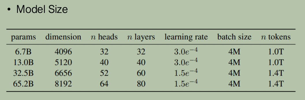
Model Size

2.2 Architecture Improvements

2.2.1 SwiGLU

• Swish 激活函数：
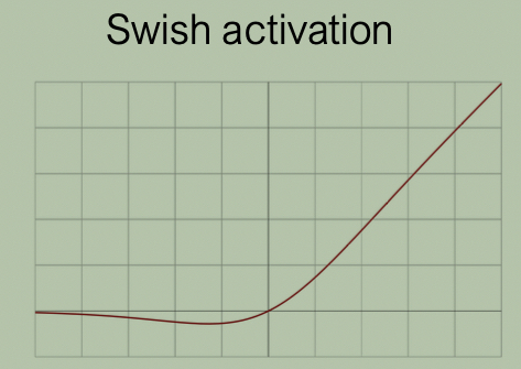
  • 公式：\(Swish(x) = x \sigma(\beta x)\)，其中 \(\sigma(x) = \frac{1}{1 + e^{-x}}\) 是 Sigmoid 函数。
  • 特点：平滑、非单调。在 PyTorch 中对应 F.silu（当 \(\beta=1\) 时）。
  • 函数图像：
  • 
• FFN with ReLU（传统结构）：
  • 公式：\(FFN(x) = max(0, x \cdot W_1 + b_1) \cdot W_2 + b_2\)
  • 隐藏层维度：\(dim = 4d\)。
• FFN with SwiGLU（LLaMA 结构）：
  • 公式：\(FFN_{SwiGLU}(x) = (Swish(x \cdot W_1 + b_1) \odot (x \cdot W_2 + b_2)) \cdot W_3 + b_2\)
  • 隐藏层维度：\(dim = \frac{2}{3} \cdot 4d\)。
  • 维度设计原因：SwiGLU 引入了额外的权重矩阵 \(W_2\)（门控分支），将隐藏层维度缩减为原来的 \(\frac{2}{3} \cdot 4d\)，以保持整体参数量与传统 ReLU FFN 大致相当。
• 与 LLaMA 源码的对应：
  • LLaMA 源码中去掉了所有 bias 项（bias=False），公式变为 \(W_3(Swish(xW_1) \odot (xW_2))\)。
  • 源码对应关系：self.w1 对应 \(W_1\)（门控），self.w3 对应 \(W_2\)（值），self.w2 对应 \(W_3\)（输出投影）。
  • 前向实现：self.w2(F.silu(self.w1(x)) * self.w3(x))。其中 F.silu 即 Swish 激活函数。

2.2.2 Rotary Position Embedding（RoPE）

• RoFormer: Enhanced Transformer with Rotary Position Embedding
• arXiv 提交日期：20 Apr 2021
• 作者苏剑林 Blog：Transformer升级之路：2、博采众长的旋转式位置编码
• 作者：
  

动机与核心思想

传统的绝对位置编码（如 Sinusoidal、可学习位置编码）直接将位置信息加到 Embedding 上，而相对位置编码往往需要修改 Attention 矩阵的计算流程，难以保持形式上的统一。

RoPE 的核心思想是：“通过绝对位置编码的形式，实现相对位置编码的效果”。

• 基本原则：让 Query 向量 \(\boldsymbol{q}_m\)（位置 \(m\)）与 Key 向量 \(\boldsymbol{k}_n\)（位置 \(n\)）的内积只依赖于两者的相对距离 \((m-n)\)，即：

\[\langle f(\boldsymbol{x}_m, m), f(\boldsymbol{x}_n, n) \rangle = g(\boldsymbol{x}_m, \boldsymbol{x}_n, m-n)\]

数学推导与原理

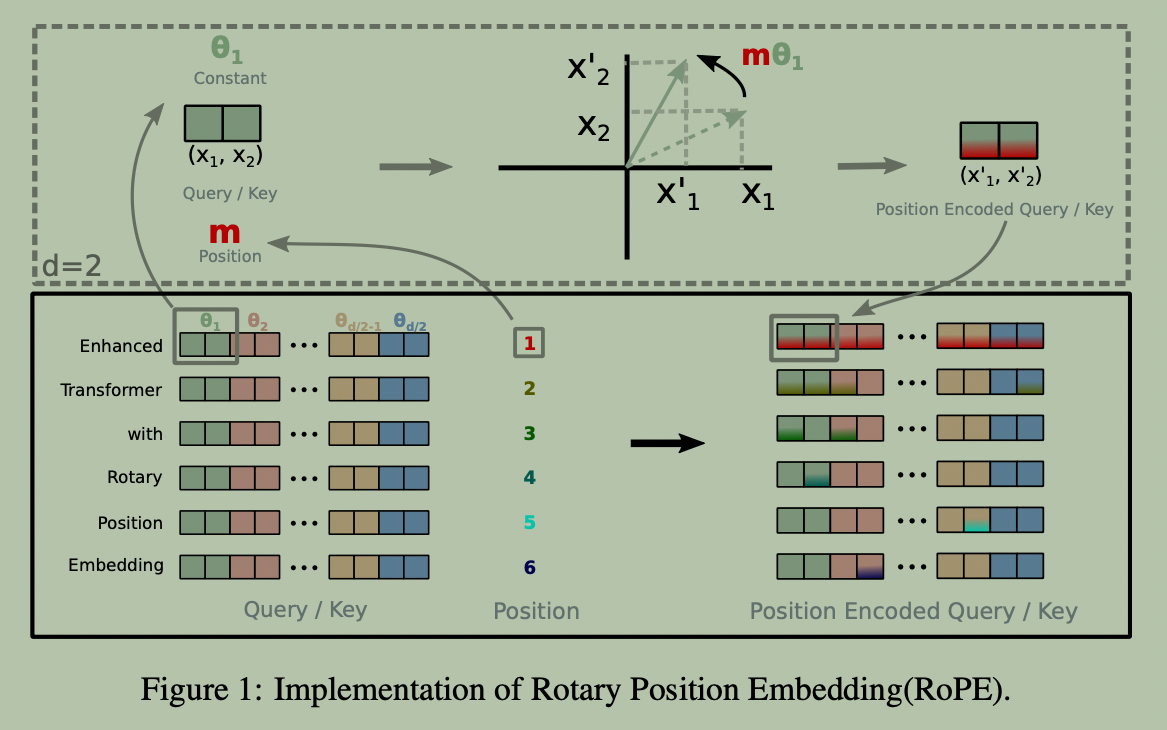
(1) 2D 基础情况

对于二维平面的特征向量 \((x_1, x_2)\)，RoPE 将位置 \(m\) 的注入表示为对向量进行角度为 \(m\theta\) 的旋转： \[f(\boldsymbol{x}_m, m) = \boldsymbol{R}_{\Theta, m}^{(2)} \boldsymbol{x}_m = \begin{pmatrix} \cos(m\theta) & -\sin(m\theta) \\ \sin(m\theta) & \cos(m\theta) \end{pmatrix} \begin{pmatrix} x_{m,1} \\ x_{m,2} \end{pmatrix}\]

• 内积性质： 在计算位置 \(m\) 的 Query 与位置 \(n\) 的 Key 的 Attention 点积时： \[f(\boldsymbol{x}_m, m)^T f(\boldsymbol{x}_n, n) = \boldsymbol{x}_m^T \boldsymbol{R}_{\Theta, m}^{T} \boldsymbol{R}_{\Theta, n} \boldsymbol{x}_n = \boldsymbol{x}_m^T \boldsymbol{R}_{\Theta, n-m} \boldsymbol{x}_n\] 这里利用了旋转矩阵的性质 \(\boldsymbol{R}_m^T \boldsymbol{R}_n = \boldsymbol{R}_{n-m}\)。绝对位置 \(m\) 和 \(n\) 在相乘后转化为相对位置差 \(n-m\)。

• 复数视角： 若将二维向量视作复数 \(\boldsymbol{x} = x_1 + \text{i}x_2\)，则旋转等价于乘以复指数 \(e^{\text{i}m\theta}\)：

\[\langle \boldsymbol{q}_m e^{\text{i}m\theta}, \boldsymbol{k}_n e^{\text{i}n\theta} \rangle = \text{Re} \left[ (\boldsymbol{q}_m e^{\text{i}m\theta}) (\boldsymbol{k}_n e^{\text{i}n\theta})^* \right] = \text{Re} \left[ \boldsymbol{q}_m \boldsymbol{k}_n^* e^{\text{i}(m-n)\theta} \right]\]

(2) 高维扩展

对于 \(d\) 维隐层向量（\(d\) 为偶数），RoPE 将 \(d\) 维空间切分为 \(d/2\) 个独立的二维子空间，每个子空间赋予不同的旋转频率 \(\theta_i\)：

\[\Theta = \{ \theta_i = 10000^{-2(i-1)/d}, \quad i \in [1, 2, \dots, d/2] \}\]

整体旋转矩阵为分块对角矩阵：

\[\boldsymbol{R}_{\Theta, m}^{(d)} = \begin{pmatrix} \cos(m\theta_1) & -\sin(m\theta_1) & 0 & 0 & \cdots & 0 & 0 \\ \sin(m\theta_1) & \cos(m\theta_1) & 0 & 0 & \cdots & 0 & 0 \\ 0 & 0 & \cos(m\theta_2) & -\sin(m\theta_2) & \cdots & 0 & 0 \\ 0 & 0 & \sin(m\theta_2) & \cos(m\theta_2) & \cdots & 0 & 0 \\ \vdots & \vdots & \vdots & \vdots & \ddots & \vdots & \vdots \\ 0 & 0 & 0 & 0 & \cdots & \cos(m\theta_{d/2}) & -\sin(m\theta_{d/2}) \\ 0 & 0 & 0 & 0 & \cdots & \sin(m\theta_{d/2}) & \cos(m\theta_{d/2}) \end{pmatrix}\]

LLaMA 代码实现

def precompute_freqs_cis(dim: int, end: int, theta: float = 10000.0):
    """
    Precompute the frequency tensor for complex exponentials (cis) with given dimensions.

    This function calculates a frequency tensor with complex exponentials using the given dimension 'dim'
    and the end index 'end'. The 'theta' parameter scales the frequencies.
    The returned tensor contains complex values in complex64 data type.

    Args:
        dim (int): Dimension of the frequency tensor.
        end (int): End index for precomputing frequencies.
        theta (float, optional): Scaling factor for frequency computation. Defaults to 10000.0.

    Returns:
        torch.Tensor: Precomputed frequency tensor with complex exponentials.

    
        

    """
    # 1. 计算每个二维子空间的旋转角频率 \theta_i (共 dim // 2 个通道)
    #    对应公式: \theta_i = 10000 ^ (-2i / d)
    #    freqs 形状: [dim // 2]    
    freqs = 1.0 / (theta ** (torch.arange(0, dim, 2)[: (dim // 2)].float() / dim))
    # 2. 生成绝对位置序列索引 m: [0, 1, 2, ..., end - 1]
    #    t 形状: [end]    
    t = torch.arange(end, device=freqs.device)  # type: ignore
    # 3. 计算外积 (Outer Product)，生成所有位置在所有通道上的旋转相位 (m * \theta_i)
    #    freqs 形状: [end, dim // 2]    
    freqs = torch.outer(t, freqs).float()  # type: ignore
    # 4. 根据极坐标生成复数张量 e^(i * m * \theta) = 1.0 * (cos(m*\theta) + i * sin(m*\theta))
    #    torch.polar(r, angle): r 是模长(全设为 1.0)，angle 是相位角
    #    freqs_cis 形状: [end, dim // 2]，数据类型自动转换为 complex64    
    freqs_cis = torch.polar(torch.ones_like(freqs), freqs)  # complex64
    return freqs_cis


def reshape_for_broadcast(freqs_cis: torch.Tensor, x: torch.Tensor):
    """
    Reshape frequency tensor for broadcasting it with another tensor.

    This function reshapes the frequency tensor to have the same shape as the target tensor 'x'
    for the purpose of broadcasting the frequency tensor during element-wise operations.

    Args:
	    # 预计算的复数频率，形状为 [seq_len, dim / 2]
        freqs_cis (torch.Tensor): Frequency tensor to be reshaped.
        #  转换成复数后的 Q 或 K 张量，形状为 [batch_size, seq_len, n_heads, dim / 2]
        x (torch.Tensor): Target tensor for broadcasting compatibility.

    Returns:
        torch.Tensor: Reshaped frequency tensor.

    Raises:
        AssertionError: If the frequency tensor doesn't match the expected shape.
        AssertionError: If the target tensor 'x' doesn't have the expected number of dimensions.
    """
    ndim = x.ndim
    assert 0 <= 1 < ndim
    # [seq_len, head_dim / 2]
    assert freqs_cis.shape == (x.shape[1], x.shape[-1])
    # 保留第 1 维 (seq_len) 和最后一维 (head_dim / 2)，其余维度补 1
    shape = [d if i == 1 or i == ndim - 1 else 1 for i, d in enumerate(x.shape)]
    # [1, seq_len, 1, head_dim / 2]
    return freqs_cis.view(*shape)


# RoPE
def apply_rotary_emb(
    xq: torch.Tensor,
    xk: torch.Tensor,
    freqs_cis: torch.Tensor,
) -> Tuple[torch.Tensor, torch.Tensor]:
    """
    Apply rotary embeddings to input tensors using the given frequency tensor.

    This function applies rotary embeddings to the given query 'xq' and key 'xk' tensors using the provided
    frequency tensor 'freqs_cis'. The input tensors are reshaped as complex numbers, and the frequency tensor
    is reshaped for broadcasting compatibility. The resulting tensors contain rotary embeddings and are
    returned as real tensors.

    Args:
        xq (torch.Tensor): Query tensor to apply rotary embeddings.
        xk (torch.Tensor): Key tensor to apply rotary embeddings.
        freqs_cis (torch.Tensor): Precomputed frequency tensor for complex exponentials.

    Returns:
        Tuple[torch.Tensor, torch.Tensor]: Tuple of modified query tensor and key tensor with rotary embeddings.

        

    """
    # 1. 转化为复数形式 (x_real + i * x_imag)
    # 形状变化过程：
    # [batch_size, seq_len, n_heads, head_dim]
    # [batch_size, seq_len, n_heads, head_dim / 2, 2]
    # [batch_size, seq_len, n_heads, head_dim / 2] （complex 类型）
    xq_ = torch.view_as_complex(xq.float().reshape(*xq.shape[:-1], -1, 2))
    xk_ = torch.view_as_complex(xk.float().reshape(*xk.shape[:-1], -1, 2))
    # 2. 调整广播形状
    freqs_cis = reshape_for_broadcast(freqs_cis, xq_)
    # 3. 复数相乘（即向量旋转），并转回实数形式 (..., d/2, 2) -> (..., d)
    # 与预计算的 e^(i * m * theta) = cos(m*theta) + i*sin(m*theta) 相乘
    #   底层自动执行：(x1 + i*x2) * (cos + i*sin)
    #   结果的实部为 (x1*cos - x2*sin)，虚部为 (x1*sin + x2*cos)
    xq_out = torch.view_as_real(xq_ * freqs_cis).flatten(3)
    xk_out = torch.view_as_real(xk_ * freqs_cis).flatten(3)
    # 4. 恢复原始的数据类型 (如 float16/bfloat16)
    return xq_out.type_as(xq), xk_out.type_as(xk)

2.3 Training

• Training Strategy
  • Trained with the standard language modeling loss function: the average log probability of all tokens without label smoothing
  • Auxiliary loss to encourage the softmax normalizer to be close to 0
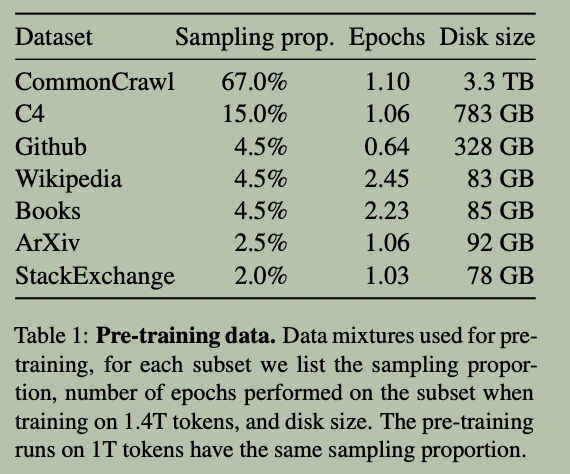
• Pre-training Details
  • Using only open-source data
  • 

3. GPT3

• Language Models are Few-Shot Learners
• arXiv 提交日期：28 May 2020
• 作者：
  

3.1 Model Architecture & Model Size

Model Architecture

• Decoder only

• With modified initialization, pre-normalization, and reversible tokenization

  • reversible tokenization: 任何文本在经过 Tokenizer 编码（Encode）成 Token ID 序列后，再通过 Decode 还原回文本时，能够做到 100% 毫无损失、无歧义地精确复原原始文本。即：
  • \[\text{Decode}(\text{Encode}(\text{Text})) \equiv \text{Text}\]

• Alternating dense and locally banded sparse attention patterns

• Sparse Attention paper

  • Generating Long Sequences with Sparse Transformers
  • arXiv 提交日期：23 Apr 2019
  • 作者：Rewon Child; Scott Gray; Alec Radford; Ilya Sutskever
    • 全部来自 OpenAI
  • 官方 blog：sparse transformer
  • 主要贡献：
    • 引入注意力矩阵的稀疏分解，降低时间空间复杂度到 \(O(n\sqrt{n})\)
    • 引入注意力矩阵重计算（recomputation of attention matrices），节省显存
    • 引入更快的 attention kernel

Attention Score Matrix 与重计算存储占用分析：

Data type	Stored	Recomputed
1024 text tokens (several paragraphs)	1.0 GB	16 MB
32x32x3 pixels (CIFAR-10 image)	9.6 GB	151 MB
64x64x3 pixels (Imagenet 64 image)	154 GB	2.4 GB
24,000 samples (~2 seconds of 12 kHz audio)	590 GB	9.2GB
由于 Attention Score 是 \(n \times n\) 矩阵，导致存储占用随着序列长度 \(n\) 呈平方增长。

Sparse Attention Motivation

Even computing a single attention matrix, however, can become impractical for very large inputs. We instead use sparse attention patterns, where each output position only computes weightings from a subset of input positions. When the subset is small relative to the full set of inputs (say, \(\sqrt{N}\) elements instead of \(N\) elements), the resulting attention computation becomes tractable even for very long sequences, with an algorithmic complexity of \(O(N\sqrt{N})\) instead of \(O(N^2)\).

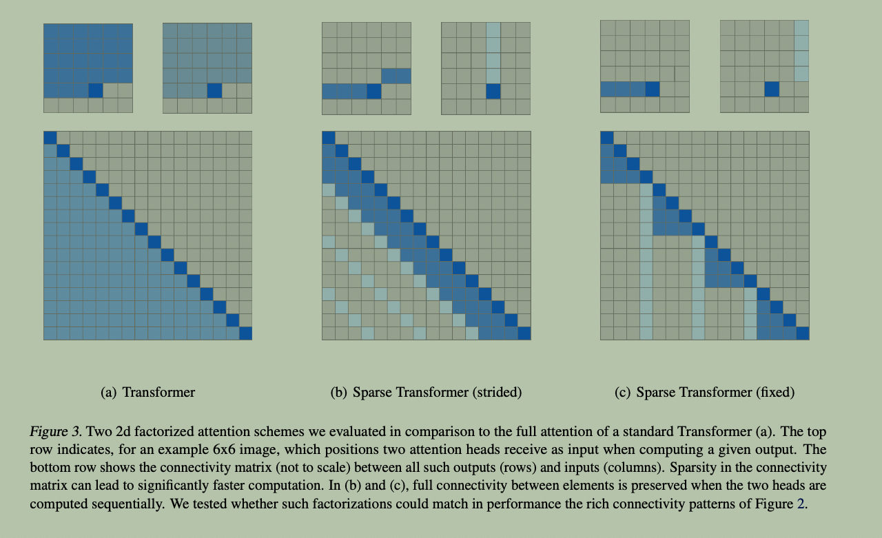
上图解释：

• 上面一行，每两个小正方形，表示两个 Attention Head 分别可以看到一个 \(6 \times 6\) 的图片的哪些像素。
• 下面一行，表示计算 Attention 时，某个输出位置可见的输入位置。
• 按列看，三列分别表示：
  • 标准 Attention：两个 head 都可以看到所有前面位置。
  • strided：一个 head 只可以看前几个位置；一个 head 可以看前面 strided 跨步的位置。
  • fixed：一个 head 可以看 block 内的前几个位置；一个 head 只可以看固定的几个位置（图中表示 block 内最后一个位置）。

历史地位与演进：

• GPT-3 论文中尝试了 Dense 与 Sparse Attention 层的交错堆叠。
• FlashAttention 随着 FlashAttention 的出现，业内重新回归 Full Attention；
• Modern Hybrid Model 目前一些模型为了应对超长上下文（如 1M+ Token）带来的 FLOPs/KV Cache容量等挑战，也采用了类似 GPT3 的 Hybrid Attention 机制：标准 Attention 与改进的 Attention 层（sliding window/linear/sparse 等各种 Attention 变体）交错。

Model Size

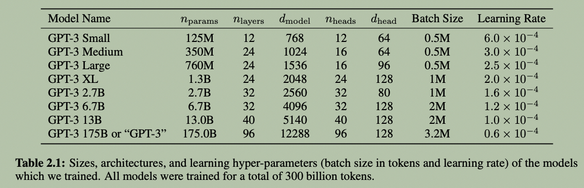
GPT-3：175B

3.2 Training

• Training Strategy
  • Unsupervised Pre-training
• Training Details
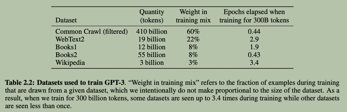
  • 数据集：
  • 
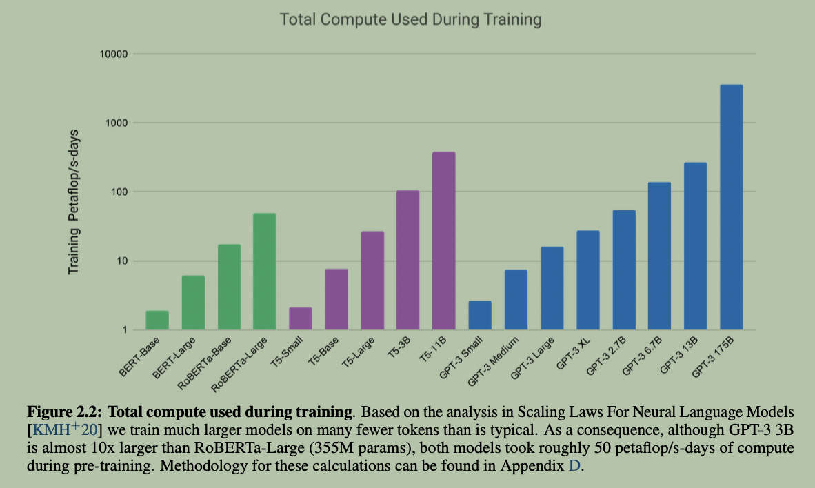
  • 训练 FLOPs：Scaling Law
  • 
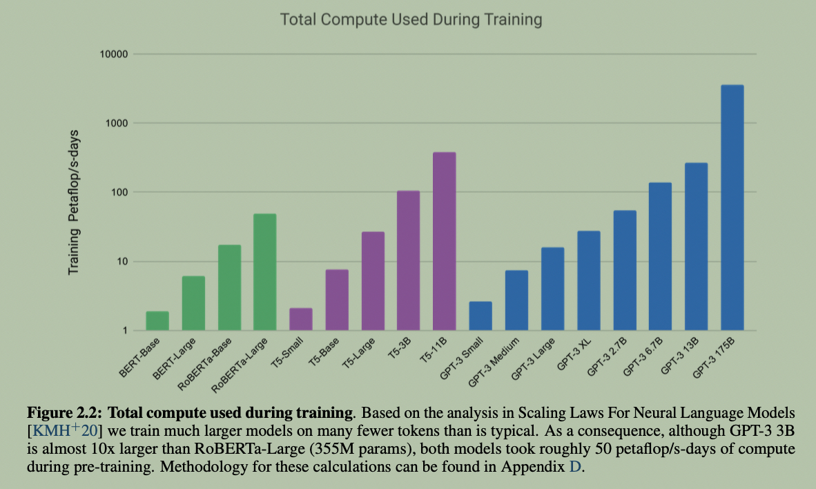
  • 上述图片对应原始数据：GPT-3 175B 训练 FLOPs 是最小的 BERT-Base 的近 2000 倍（1925.93）。
  • 

4. Summary

• Pretraining: Mask-labeled recovery of random spans + next token prediction
• Multitask supervised fine-tuning with instruction templates
  • T5, InstructGPT
• Relative position: Rotary positional embedding
• Smooth activation: SwishGLU
• Sparse attention