LLM Systems Assignment 2: Minitorch Framework

本次 homework 需要编写的代码量实际上非常少(100 行左右),完成作业的关键是理解 minitorch 设计和已有代码。因此,本文主要介绍 minitorch 代码结构,解释其 Tensor、Parameter、Operator、Module、History 等关键设计和实现。

课程官方对 minitorch 有个 Jupyter Notebook 做了详细介绍可参考。本文内容基于 homework 2 代码框架和上述 Jupyter Notebook 内容。

1. Architecture


minitorch 整体组织是一个明显的分层结构:

1
2
3
4
5
6
7
8
9
10
11
12
13
14
15
16
┌────────────────────────────────────────────────────┐
│ project/run_sentiment.py 应用层:训练循环、数据编码 │
├────────────────────────────────────────────────────┤
│ module.py / optim.py / nn.py NN 层:Module 树、 │
│ Parameter、SGD/Adam │
├────────────────────────────────────────────────────┤
│ tensor.py / tensor_functions.py 计算图层:Tensor、 │
│ History、Function │
├────────────────────────────────────────────────────┤
│ tensor_ops.py 后端层:map/zip/reduce 三类高阶算子组合 │
│ SimpleOps(纯 Python)或 │
│ CudaKernelOps(HW1 的 CUDA kernel) │
├────────────────────────────────────────────────────┤
│ tensor_data.py / operators.py 数据层:存储、shape、 │
│ strides、标量函数 │
└────────────────────────────────────────────────────┘

关键模块包括:

  • Tensor
    • tensor 数据存储
    • 计算图表示
  • Function
    • Operator
    • forward/backward 计算过程实现
  • Module
    • Parameter
    • 参数初始化
    • Module 可组合构成神经网络结构
  • Optimizer
    • 与 Module 的参数交互

模块与代码文件对应关系说明如下:

1
2
3
4
5
6
7
8
9
10
11
12
13
14
15
16
17
18
19
20
21
22
23
24
25
# 输出省略了部分文件
$ git ls-files | tree --fromfile
.
|-- minitorch
| |-- autodiff.py # 自动求导相关代码,homework 2_1 todo 位置
| |-- cuda_kernel_ops.py # CUDA backend op Python 接口,本次 homework 忽略
| |-- datasets.py # mock 数据集(二维点到 label)生成,本次 homework 忽略
| |-- module.py # Module & Parameter 实现
| |-- nn.py # dropout 等简单&常用神经网络模块实现
| |-- operators.py # Python 实现的 element-wise add/mult 等 op
| |-- optim.py # 优化器实现,提供了 SGD 和 Adam
| |-- tensor.py # Tensor 实现,计算基本单位和计算图的组成单元
| |-- tensor_data.py # Tensor 存储层实现,shape + strides + 连续存储表示法
| |-- tensor_functions.py # Function 基类(前向建图机制,apply)与常用 op 的 fwd/bwd 配对实现;常用 Tensor 工厂函数实现(zeros/ones/rand 等)
| |-- tensor_ops.py # 基于 operators.py 封装为 TensorOps 与 TensorBackend,Tensor 持有 TensorBackend 作为成员供 Function 调用
| `-- testing.py
|-- project
| `-- run_sentiment.py # homework 2_2 2-3 位置,实现网络结构与训练 main loop
|-- src
| `-- combine.cu # CUDA kernel 实现,本 homework 忽略
`-- tests
|-- strategies.py
|-- tensor_strategies.py # 测试
|-- test_neural_network.py
`-- test_tensor_autodiff.py

2. Data Storage and Operators

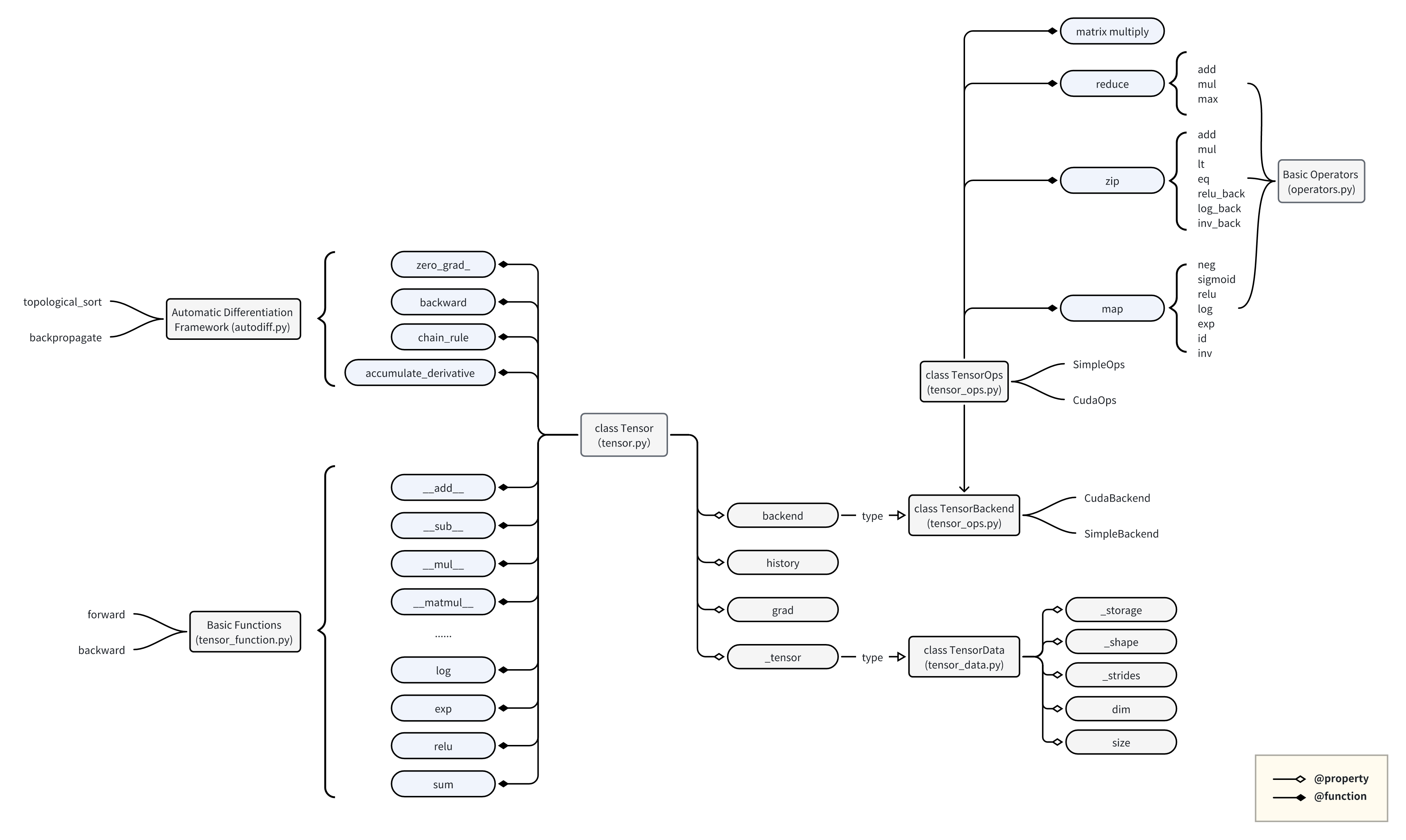
首先看下 class Tensor 如何与其他模块关联起来,包括:

  • 数据存储 class TensorData
  • 计算后端 class TensorBackend
    • 依赖 class TensorOps 来对不同的 operators 执行实际计算
    • class Function 及其实现类抽象并实现了基础运算


上图以中间的 class Tensor 为核心,整体分为以下几个部分:

  • 左上角:自动求导相关方法,包括:反向传播、链式法则等。
  • 左下角:Tensor 支持的相关运算,基于 class Function 实现计算图构建和每个 op 的 bwd 实现。
  • 右侧 backend:class TensorBackend 类型,基于 TensorOps 支持 map、zip、reduce、matrix multiply 四大类运算。
  • 右侧 _tensor:Tensor 底层存储,class TensorData 实现。

接下来,开始自底向上看下 TensorStorage 、TensorOps 与 TensorBackend 代码。

2.1 TensorData

1
2
3
4
5
6
7
8
9
10
11
12
13
14
15
16
17
18
19
20
21
22
23
24
25
26
27
28
29
30
31
32
33
34
35
36
37
38
39
40
41
42
43
44
45
46
47
48
49
50
51
52
53
54
55
56
57
58
59
60
61
62
63
64
65
66
67
68
69
70
71
72
73
74
75
76
77
78
79
80
81
82
83
84
85
86
87
88
89
90
91
92
93
94
95
96
97
98
99
100
101
102
103
104
105
106
107
108
109
110
111
112
113
114
115
116
117
118
119
120
121
122
123
124
from __future__ import annotations

import random
from typing import Iterable, Optional, Sequence, Tuple, Union

import numba
from numba import cuda
import numpy as np
import numpy.typing as npt
from numpy import array, float64
from typing_extensions import TypeAlias

from .operators import prod

MAX_DIMS = 32


class IndexingError(RuntimeError):
"Exception raised for indexing errors."
pass

datatype = np.float32

# type alias
# 使用 numpy NDArray 作为 tensor 底层存储
Storage: TypeAlias = npt.NDArray[datatype]
OutIndex: TypeAlias = npt.NDArray[np.int32]
Index: TypeAlias = npt.NDArray[np.int32]
Shape: TypeAlias = npt.NDArray[np.int32]
Strides: TypeAlias = npt.NDArray[np.int32]

# 这里 type alias 分为两套:
# - 面向用户的 Python 层 tuple/list 等
# - TensorData 内部的使用 np.array 连续存储的版本
UserIndex: TypeAlias = Sequence[int]
UserShape: TypeAlias = Sequence[int]
UserStrides: TypeAlias = Sequence[int]

# 一些辅助函数,逻辑和 homework 1 内 GPU device 实现一致,这里只贴签名
def index_to_position(index: Index, strides: Strides) -> int:
pass

def to_index(ordinal: int, shape: Shape, out_index: OutIndex) -> None:
pass

def broadcast_index(

big_index: Index, big_shape: Shape, shape: Shape, out_index: OutIndex

) -> None:
pass

def shape_broadcast(shape1: UserShape, shape2: UserShape) -> UserShape:
pass

def strides_from_shape(shape: UserShape) -> UserStrides:
pass


class TensorData:
_storage: Storage
_strides: Strides
_shape: Shape
strides: UserStrides
shape: UserShape
dims: int

def __init__(
self,
storage: Union[Sequence[float], Storage],
shape: UserShape,
strides: Optional[UserStrides] = None,
):
if isinstance(storage, np.ndarray):
# 直接传入 np.array,仅进行类型转换
self._storage = storage.astype(datatype)
else:
# 传入 list,构造为 np.array 并进行类型转换
self._storage = array(storage, dtype=datatype)

if strides is None:
# 默认 row-major layout
strides = strides_from_shape(shape)

assert isinstance(strides, tuple), "Strides must be tuple"
assert isinstance(shape, tuple), "Shape must be tuple"
if len(strides) != len(shape):
raise IndexingError(f"Len of strides {strides} must match {shape}.")
# 构造传入的 shape/strides 全部转换为 np.array
self._strides = array(strides)
self._shape = array(shape)
# user 版本 list/tuple 也保存一份
self.strides = strides
self.dims = len(strides)
self.size = int(prod(shape))
self.shape = shape
assert len(self._storage) == self.size

def tuple(self) -> Tuple[Storage, Shape, Strides]:
return (self._storage, self._shape, self._strides)

# 省略部分方法,核心是理解 shape & strides & contiguous_storage Tensor 表示法

def permute(self, *order: int) -> TensorData:
"""
Permute the dimensions of the tensor.

Args:
*order: a permutation of the dimensions

Returns:
New `TensorData` with the same storage and a new dimension order.
"""
assert list(sorted(order)) == list(
range(len(self.shape))
), f"Must give a position to each dimension. Shape: {self.shape} Order: {order}"

# 以 permute 方法为例,说明 shape & strides 表示法优点:
# 进行 permute 操作时无任何 storage 层拷贝,只需要根据传入参数 order 重新排列 shape & strides 即可
return TensorData(
self._storage,
tuple([self.shape[o] for o in order]),
tuple([self._strides[o] for o in order]),
)

这里先提前看下 class Tensor 中与 TensorData 有关的部分:

1
2
3
4
5
6
7
8
9
10
11
12
13
14
15
16
17
18
19
20
21
22
23
24
25
26
27
28
29
30
31
32
33
34
35
36
37
38
39
40
41
42
43
44
45
46
47
48
49
50
51
52
53
54
55
56
57
58
59
60
61
62
63
64
65
66
67
68
69
70
71
72
73
74
75
76
77
class Tensor:
"""
Tensor is a generalization of Scalar in that it is a Variable that
handles multidimensional arrays.
"""

backend: TensorBackend
history: Optional[History]
grad: Optional[Tensor]
# Tensor 底层存储委托给 TensorData
_tensor: TensorData
unique_id: int
name: str

def __init__(
self,
v: TensorData,
back: Optional[History] = None,
name: Optional[str] = None,
backend: Optional[TensorBackend] = None,
):
global _tensor_count
_tensor_count += 1
self.unique_id = _tensor_count
assert isinstance(v, TensorData)
assert backend is not None
self._tensor = v
self.history = back
self.backend = backend
self.grad = None
if name is not None:
self.name = name
else:
self.name = str(self.unique_id)

self.f = backend

# Tensor 的一些接口直接映射到 TensorData 的接口
# Properties
@property
def shape(self) -> UserShape:
"""
Returns:
shape of the tensor
"""
return self._tensor.shape

@property
def size(self) -> int:
"""
Returns:
int : size of the tensor
"""
return self._tensor.size

@property
def dims(self) -> int:
"""
Returns:
int : dimensionality of the tensor
"""
return self._tensor.dims

# 后面介绍 TensoOps 会用到
def tuple(self) -> Tuple[Storage, Shape, Strides]:
return self._tensor.tuple()

# 工厂方法
@staticmethod
def make(
storage: Union[Storage, List[float]],
shape: UserShape,
strides: Optional[UserStrides] = None,
backend: Optional[TensorBackend] = None,
) -> Tensor:
"Create a new tensor from data"
return Tensor(TensorData(storage, shape, strides), backend=backend)

2.2 TensorOps & Operators

首先看简单的 operators.py,其内部主要是一些简单的一元或二元函数实现:

1
2
3
4
5
6
7
8
9
10
11
12
13
14
15
16
17
18
19
20
21
22
23
24
25
26
27
28
29
30
31
32
33
34
35
36
37
38
39
40
41
42
43
44
45
46
47
48
49
50
51
52
53
54
55
56
57
58
59
60
61
62
63
64
65
66
67
68
69
"""
Collection of the core mathematical operators used throughout the code base.
"""

import math
from typing import Callable, Iterable


def pow(x: float, y: float) -> float:
return x ** y


def tanh(x: float) -> float:
return math.tanh(x)


def mul(x: float, y: float) -> float:
"$f(x, y) = x * y$"
return x * y


def id(x: float) -> float:
"$f(x) = x$"
return x


def add(x: float, y: float) -> float:
"$f(x, y) = x + y$"
return x + y


def neg(x: float) -> float:
"$f(x) = -x$"
return -x

# 省略部分

# 列出部分和反向传播相关的(但是只是 element-wise 函数实现,供上层调用)
EPS = 1e-6

def log(x: float) -> float:
"$f(x) = log(x)$"
return math.log(x + EPS)


def exp(x: float) -> float:
"$f(x) = e^{x}$"
return math.exp(x)


# 这里即利用了链式法则:复合函数导数为 d 乘以 log 函数(自然对数)的导数
def log_back(x: float, d: float) -> float:
r"If $f = log$ as above, compute $d \times f'(x)$"
return d / (x + EPS)


def inv(x: float) -> float:
"$f(x) = 1/x$"
return 1.0 / x


def inv_back(x: float, d: float) -> float:
r"If $f(x) = 1/x$ compute $d \times f'(x)$"
return -(1.0 / x**2) * d


def relu_back(x: float, d: float) -> float:
r"If $f = relu$ compute $d \times f'(x)$"
return d if x > 0 else 0.0

基于上述简单的 operator 实现,上层进一步封装为 TensorOps 与 TensorBackend。

首先看 TensorOps,其实际上只是一个简单的接口:

1
2
3
4
5
6
7
8
9
10
11
12
13
14
15
16
17
18
19
20
21
22
23
class MapProto(Protocol):
def __call__(self, x: Tensor, out: Optional[Tensor] = ..., /) -> Tensor:
...


class TensorOps:
@staticmethod
def map(fn: Callable[[float], float]) -> MapProto:
pass

@staticmethod
def zip(fn: Callable[[float, float], float]) -> Callable[[Tensor, Tensor], Tensor]:
pass

@staticmethod
def reduce(
fn: Callable[[float, float], float], start: float = 0.0
) -> Callable[[Tensor, int], Tensor]:
pass

@staticmethod
def matrix_multiply(a: Tensor, b: Tensor) -> Tensor:
raise NotImplementedError("Not implemented in this assignment")

包括 4 个方法:

  • map:输入为一元函数,输出为一个可调用对象,输入输出都是一个 Tensor。
  • zip:输入为二元函数,输出为一个可调用对象,接受两个 Tensor 参数返回一个 Tensor 参数。
  • reduce:输入为二元函数,输出为一个可调用对象,接受一个 Tenso 和一个 int 参数,返回 Tenso 参数。
  • matrix_multiply:矩阵乘法。

然后来看 SimpleOps 的实现:

1
2
3
4
5
6
7
8
9
10
11
12
13
14
15
16
17
18
19
20
21
22
23
24
25
26
27
28
29
30
31
32
33
34
35
36
37
38
39
40
41
42
43
44
45
46
47
48
49
50
51
52
53
54
55
56
57
58
59
60
61
62
63
64
65
66
67
68
69
70
71
72
73
74
75
76
77
78
79
80
81
82
83
84
85
86
87
88
89
90
91
92
93
94
95
96
class SimpleOps(TensorOps):
@staticmethod
def map(fn: Callable[[float], float]) -> MapProto:
# 调用下面的 `tensor_map(fn)`
f = tensor_map(fn)

def ret(a: Tensor, out: Optional[Tensor] = None) -> Tensor:
if out is None:
out = a.zeros(a.shape)
# 前面介绍过的 tuple() 方法,返回 Tensor 的 storage/shape/strides
f(*out.tuple(), *a.tuple())
return out

return ret

@staticmethod
def zip(
fn: Callable[[float, float], float]
) -> Callable[["Tensor", "Tensor"], "Tensor"]:
# 略

@staticmethod
def reduce(
fn: Callable[[float, float], float], start: float = 0.0
) -> Callable[["Tensor", int], "Tensor"]:
# 略

@staticmethod
def matrix_multiply(a: "Tensor", b: "Tensor") -> "Tensor":
# 略

is_cuda = False


# 该函数核心功能:将 element-wise fn 封装为一个接受 Tensor 的 Storage/Shape/Strides 作为参数的可调用对象
# 值得一提的是,这里的可调用对象参数要求是 np.array,而不是 Python 原生类型
def tensor_map(
fn: Callable[[float], float]
) -> Callable[[Storage, Shape, Strides, Storage, Shape, Strides], None]:
"""
Low-level implementation of tensor map between
tensors with *possibly different strides*.

Simple version:

* Fill in the `out` array by applying `fn` to each
value of `in_storage` assuming `out_shape` and `in_shape`
are the same size.

Broadcasted version:

* Fill in the `out` array by applying `fn` to each
value of `in_storage` assuming `out_shape` and `in_shape`
broadcast. (`in_shape` must be smaller than `out_shape`).

Args:
fn: function from float-to-float to apply

Returns:
Tensor map function.
"""

def _map(
out: Storage,
out_shape: Shape,
out_strides: Strides,
in_storage: Storage,
in_shape: Shape,
in_strides: Strides,
) -> None:
out_index: Index = np.zeros(MAX_DIMS, np.int16)
in_index: Index = np.zeros(MAX_DIMS, np.int16)
for i in range(len(out)):
# 处理 index 映射广播等
to_index(i, out_shape, out_index)
broadcast_index(out_index, out_shape, in_shape, in_index)
o = index_to_position(out_index, out_strides)
j = index_to_position(in_index, in_strides)
# 调用传入的 fn 函数
out[o] = fn(in_storage[j])

return _map


def tensor_zip(
fn: Callable[[float, float], float]
) -> Callable[
[Storage, Shape, Strides, Storage, Shape, Strides, Storage, Shape, Strides], None
]:
pass


def tensor_reduce(
fn: Callable[[float, float], float]
) -> Callable[[Storage, Shape, Strides, Storage, Shape, Strides, int], None]:
pass

原始代码的注释实际上已经非常清晰,这里为了篇幅删掉了大部分,仅保留最简单的 map 实现相关注释。实际上,为了实现 TensorOps,minitorch 从三个层次进行了自底向上的组织与实现:

  • 最底层(最简单)的 element-wise function 实现,在 operators.py 中实现。
  • 中间层的 tensor_map/zip/reduce 接受参数是一个 element-wise func,返回一个 storage/shape/strides 作为输入参数的可调用对象,进行 Tensor 级别的全部元素的处理。
  • SimpleOps 提供接口接受 element-wise func 作为输入参数,返回将 Tensor 作为输入参数的可调用对象,内部获取 Tensor 的 storage/shape/strides 元组,调用中间层的接口。
  • 三层最核心的区别:
    • 最底层:普通标量作为参数,返回标量。
    • 中间层:storage/shape/strides 作为参数,同时处理可能的广播。
    • 最上层:Tensor 进行参数,可能预先进行返回值 Tensor 构造。

真正暴露到其他模块,供 class Tensor 使用的接口实际上是 class TensorBackend:

1
2
3
4
5
6
7
8
9
10
11
12
13
14
15
16
17
18
19
20
21
22
23
24
25
26
27
28
29
30
31
32
33
34
35
36
37
38
39
40
41
class TensorBackend:
def __init__(self, ops: Type[TensorOps]):
"""
Dynamically construct a tensor backend based on a `tensor_ops` object
that implements map, zip, and reduce higher-order functions.

Args:
ops : tensor operations object see `tensor_ops.py`


Returns :
A collection of tensor functions

"""

# Maps
self.neg_map = ops.map(operators.neg)
self.sigmoid_map = ops.map(operators.sigmoid)
self.relu_map = ops.map(operators.relu)
self.log_map = ops.map(operators.log)
self.exp_map = ops.map(operators.exp)
self.id_map = ops.map(operators.id)
self.inv_map = ops.map(operators.inv)
self.tanh_map = ops.map(operators.tanh)

# Zips
self.add_zip = ops.zip(operators.add)
self.mul_zip = ops.zip(operators.mul)
self.lt_zip = ops.zip(operators.lt)
self.eq_zip = ops.zip(operators.eq)
self.is_close_zip = ops.zip(operators.is_close)
self.relu_back_zip = ops.zip(operators.relu_back)
self.log_back_zip = ops.zip(operators.log_back)
self.inv_back_zip = ops.zip(operators.inv_back)
self.pow_scalar_zip = ops.zip(operators.pow)

# Reduce
self.add_reduce = ops.reduce(operators.add, 0.0)
self.mul_reduce = ops.reduce(operators.mul, 1.0)
self.matrix_multiply = ops.matrix_multiply
self.cuda = ops.cuda

在理解了前面的代码后,这个 TensorBackend 实现就显得尤为简单了:调用 TensorOps 提供的接口,传入 operators.py 内的 func,注册 Tensor 级别的运算接口。

2.3 Connect to CUDA Kernels

CUDA 相关支持的代码在:

  • minitorch/cuda_kernel_ops.py
  • src/combine.cu

这两个文件的关系为:

  • .cu 文件提供了 Tensor(storage/shape/strides)作为输入参数的接口,内部调用实现的 CUDA kernel,从而实现在 GPU 上完成相关 operator。该源文件使用 nvcc 编译成 .so 文件,供 Python 层调用相关接口。
  • .py 文件使用 pycuda 库打开 .so 文件,传入 Tensor 的 storage/shape/strides 作为输入参数(注意,这里传入的参数必须是 TensorData 内 np.array 版本的,因为底层 C++ 接口要求连续存储)调用 .cu 文件实现的接口。

3. Automatic Differentiation

理解自动求导如何实现,关键在两点:

  • forward 时如何构建计算图?
    • 如何区分 Tensor 是否需要梯度?是否是可学习的 Parameter?
    • 如何记录中间 Tensor 的来源(Function),以在反向传播时计算梯度?
  • backward 时如何从 loss 开始进行反向传播?
    • 链式法则如何实现?
    • 反向传播顺序(homework 中的拓扑排序)如何保证?

3.1 Element-wise Multiply Forward 调用路径

再次看 Tensor 的相关代码:

1
2
3
4
5
6
7
8
9
10
11
12
13
14
15
16
17
18
19
20
21
22
23
24
25
26
27
28
29
30
31
32
33
34
35
36
37
38
39
40
41
42
43
44
45
46
47
48
49
50
51
52
53
54
55
56
57
58
59
60
61
62
63
64
65
66
67
68
69
70
71
72
73
74
75
76
77
78
79
80
81
82
83
84
85
86
87
88
89
90
91
92
93
94
95
96
97
98
99
100
101
102
103
104
105
class Tensor:
"""
Tensor is a generalization of Scalar in that it is a Variable that
handles multidimensional arrays.
"""

backend: TensorBackend
history: Optional[History]
grad: Optional[Tensor]
_tensor: TensorData
unique_id: int
name: str

def __init__(
self,
v: TensorData,
back: Optional[History] = None,
name: Optional[str] = None,
backend: Optional[TensorBackend] = None,
):
global _tensor_count
_tensor_count += 1
self.unique_id = _tensor_count
assert isinstance(v, TensorData)
assert backend is not None
self._tensor = v
self.history = back
self.backend = backend
self.grad = None
if name is not None:
self.name = name
else:
self.name = str(self.unique_id)

self.f = backend

def requires_grad_(self, x: bool) -> None:
if x:
self.history = History()
else:
self.history = None

# 省略很多方法,先仅考虑这里的 element-wise multiply
def __mul__(self, b: TensorLike) -> Tensor:
return Mul.apply(self, self._ensure_tensor(b))


# 清空 Tensor 的 history,保留 TensorData 引用,生成一个 is_constant() 的节点
def detach(self) -> Tensor:
return Tensor(self._tensor, backend=self.backend)

# Variable elements for backprop

def accumulate_derivative(self, x: Any) -> None:
"""
Add `val` to the the derivative accumulated on this variable.
Should only be called during autodifferentiation on leaf variables.

Args:
x : value to be accumulated
"""
# 叶子节点梯度累加
assert self.is_leaf(), "Only leaf variables can have derivatives."
if self.grad is None:
self.grad = Tensor.make(
[0] * int(operators.prod(self.shape)), self.shape, backend=self.backend
)
self.grad += x

def is_leaf(self) -> bool:
"True if this variable created by the user (no `last_fn`)"
return self.history is not None and self.history.last_fn is None

def is_constant(self) -> bool:
return self.history is None

@property
def parents(self) -> Iterable[Variable]:
assert self.history is not None
return self.history.inputs

def chain_rule(self, d_output: Any) -> Iterable[Tuple[Variable, Any]]:
h = self.history
assert h is not None
assert h.last_fn is not None
assert h.ctx is not None

x = h.last_fn._backward(h.ctx, d_output)
assert len(x) == len(h.inputs), f"Bug in function {h.last_fn}"
return [
(inp, inp.expand(self._ensure_tensor(d_in)))
for inp, d_in in zip(h.inputs, x)
]

def backward(self, grad_output: Optional[Tensor] = None) -> None:
if grad_output is None:
assert self.shape == (1,), "Must provide grad_output if non-scalar"
grad_output = Tensor.make([1.0], (1,), backend=self.backend)
backpropagate(self, grad_output)

def zero_grad_(self) -> None: # pragma: no cover
"""
Reset the derivative on this variable.
"""
self.grad = None

对于两个 Tensor 的 a * b 操作,将调用上述 __mul__ 方法,相关代码如下:

minitorch/tensor_functions.py

1
2
3
4
5
6
7
8
9
10
11
12
13
14
15
16
17
18
19
20
21
22
23
24
25
26
27
28
29
30
31
32
33
34
35
36
37
38
39
40
41
42
43
44
45
46
47
48
49
50
51
52
53
54
55
56
57
58
59
60
61
62
63
64
65
66
67
68
69
70
71
72
73
74
75
76
77
78
79
@dataclass
class History:
"""
`History` stores the history of `Function` operations that was
used to construct the current Variable.
"""

last_fn: Optional[Type[Function]] = None
ctx: Optional[Context] = None
inputs: Sequence[Tensor] = ()


@dataclass
class Context:
"""
Context class is used by `Function` to store information during the forward pass.
"""

no_grad: bool = False
saved_values: Tuple[Any, ...] = ()

def save_for_backward(self, *values: Any) -> None:
"Store the given `values` if they need to be used during backpropagation."
if self.no_grad:
return
self.saved_values = values

@property
def saved_tensors(self) -> Tuple[Any, ...]:
return self.saved_values

# Constructors
class Function:
@classmethod
def _backward(cls, ctx: Context, grad_out: Tensor) -> Tuple[Tensor, ...]:
return wrap_tuple(cls.backward(ctx, grad_out)) # type: ignore

@classmethod
def _forward(cls, ctx: Context, *inps: Tensor) -> Tensor:
return cls.forward(ctx, *inps) # type: ignore

@classmethod
def apply(cls, *vals: Tensor) -> Tensor:
raw_vals = []
need_grad = False
for v in vals:
if v.requires_grad():
need_grad = True
raw_vals.append(v.detach())

# Create the context.
ctx = Context(not need_grad)

# Call forward with the variables.
c = cls._forward(ctx, *raw_vals)
# assert isinstance(c, Tensor), "Expected return type Tensor got %s" % (
# type(c)
# )

# Create a new variable from the result with a new history.
back = None
if need_grad:
back = minitorch.History(cls, ctx, vals)
return minitorch.Tensor(c._tensor, back, backend=c.backend)


class Mul(Function):
@staticmethod
def forward(ctx: Context, a: Tensor, b: Tensor) -> Tensor:
ctx.save_for_backward(a, b)
return a.f.mul_zip(a, b)

@staticmethod
def backward(ctx: Context, grad_output: Tensor) -> Tuple[Tensor, Tensor]:
a, b = ctx.saved_values
return (
grad_output.f.mul_zip(b, grad_output),
grad_output.f.mul_zip(a, grad_output),
)

首先看 class Mul(Function) 的 forward 与 backward 方法:

  • forward:保存输入 Tensor a/b 供 backward 时使用,然后使用 TensorBackend 内注册的 op 进行计算,返回结果 Tensor(此时的 Tensor 仅完成了纯数学上的计算,还没有进行计算图相关操作)。
  • backward:提取保存的输入 Tensor a/b,调用相应 op 进行链式法则梯度计算。

然后看接口 class Function 的 apply 方法,其调用了实现类的 forward 方法并构建计算图。

  • 遍历输入 Tensor,如果其中一个需要梯度,那么结果 Tensor 也需要计算梯度。同时调用 detach() 方法,获取输入 Tensor 的一个 constant 视图。
  • 构造 Context 对象,传入是否需要梯度参数。
  • 调用实现类 forward 方法,完成前向计算。
  • 如果需要计算梯度,构造 History 对象(否则为 None),保存 Function class、context 以及输入 Tensor 列表,供 backward 时使用。class History 包括三个成员:
    • last_fn:计算结果 Tensor 由哪个 Function 计算出来,用于链式法则计算梯度。
    • ctx:保存计算梯度需要用到的 Tensor,通常需要保存输入 Tensor 以及部分中间计算结果,供 backward 时使用以让 backward 实现更加简洁。ctx 内保存到 Tensor 是 detach 之后的纯数值引用,无计算图相关成员。
    • inputs:保存计算得到该 Tensor 的所有输入 Tensor。这里保存的 Tensor 是带有 history 成员的携带计算图历史的原始输入 Tensor,不同于 ctx 中 detach 后的 Tensor。class Tensor 的 parents() 方法即返回 self.history.inputs,autodiff.py 内待实现的的 topological_sort 函数最终调用的就是 Tensor 的相关方法。
    • ctx 与 inputs 保存的 Tensor 分别服务于两个目的:
      • 纯数值计算
      • 计算图构建
    • 下文称这个特性为 ctx 双通道
  • 根据数值计算结果 Tensor 和 History 对象,返回最终的结果 Tensor,进行可能的计算图构建。

至此,我们已经梳理了 forward 过程中计算图是如何构建的。现在,用代码和简单图示再展示上述过程,以帮助理解:

1
2
3
4
5
6
7
8
9
10
11
12
13
14
15
16
17
18
19
20
21
22
23
import minitorch

backend = minitorch.TensorBackend(minitorch.SimpleOps)

# ── 1. 构造参数与输入 ──────────────────────────────────────────────
# w 是可学习参数:requires_grad_(True) 挂一个空 History{},
# 使其成为 is_leaf() 为 True 的"叶子节点"(梯度的最终目的地)
w = minitorch.tensor([2.0], backend=backend)
w.requires_grad_(True)

# x 是输入数据:不挂 History,是 is_constant() 的常量节点
x = minitorch.tensor([3.0], backend=backend)
y_true = minitorch.tensor([10.0], backend=backend)

# ── 2. 前向计算:每一步运算都触发 Function.apply 建图 ──────────────
z = w * x # → Mul.apply(w, x):数值 6.0,挂 History(Mul, ctx, (w, x))
diff = z - y_true # → Add.apply(z, -y_true):数值 -4.0,挂 History(Add, ...)
loss = diff * diff # → Mul.apply(diff, diff):数值 16.0,注意 diff 被引用两次!

# ── 3. 反向传播 ────────────────────────────────────────────────────
loss.backward() # → backpropagate(loss, 1.0)

print(w.grad) # 2 * diff * x = 2 * (-4) * 3 = -24.0 ✓ 可手算验证

先只考虑上述代码 forward 过程,loss 计算完成后,Tensor 的相关成员引用关系如下:

1
2
3
4
5
6
7
8
9
10
11
12
13
14
15
16
17
18
19
20
21
22
23
24
25
26
27
28
29
30
31
32
33
34
35
36
37
38
39
40
41
42
43
44
┌─────────────────────────────────────────────────────────────────┐
│ loss: Tensor │
│ history = History( │
│ last_fn = Mul ← "我是被谁算出来的" │
│ ctx = Context( ← detach 影子通道(纯数值) │
│ no_grad = False │
│ saved_values = (diff_detached, diff_detached) │
│ ) 影子 history=None,链在此截断 ✂ │
│ inputs = (diff, diff) ← 原始节点通道(梯度调度用) │
│ ) │
│ grad = None │
└─────────────────────────────────────────────────────────────────┘
│ history.inputs(即 parents 属性返回的东西)
▼
┌─────────────────────────────────────────────────────────────────┐
│ diff: Tensor │
│ history = History( │
│ last_fn = Add │
│ ctx.saved_values = (z_detached, y_true_detached) │
│ inputs = (z, y_true) │
│ ) │
│ grad = None(中间节点,梯度路过不停留) │
└─────────────────────────────────────────────────────────────────┘
│ │
▼ ▼
┌──────────────────────────┐ ┌──────────────────────────┐
│ z: Tensor │ │ y_true: 常量 │
│ history = History( │ │ history = None │
│ last_fn = Mul │ │ is_constant() == True │
│ ctx.saved = (wd, xd) │ │ backward 时被跳过 │
│ inputs = (w, x) │ │ │
│ ) │ │ │
└──────────────────────────┘ └──────────────────────────┘
│
├──────────────┬─────────────────────────┐
▼ ▼ ▼
┌────────────────────┐ ┌────────────────────────┐
│ w: 叶子节点 │ │ x: 常量输入 │
│ history = Hist( │ │ history = None │
│ last_fn=None) │ │ is_constant()==True │
│ is_leaf()=True │ │ │
│ grad = -24.0 ◄───┼──────────┼── backward 的终点 │
│ (梯度落账处) │ │ (无 grad 槽位) │
└────────────────────┘ └────────────────────────┘

摘出上述 Tensor 引用关系,仅看计算图如下:

1
2
3
4
5
6
7
8
9
10
11
12
13
w(leaf)      x(const)      y_true(const)
│ │ │
└── Mul ─────┘ │ ← z.history: last_fn=Mul
│ │
z │
│ │
└── Add ────────────────┘ ← diff.history: last_fn=Add
│
diff ──┐
│ (diff 出现两次)
└── Mul ┘ ← loss.history: last_fn=Mul
│
loss ← backward(grad=1.0) 从这里出发,逆着箭头走

上图实际上也提到了 backward 过程,后文会详细介绍。不过实际上,理解了 forward 建图过程,backward 实现也就比较容易理解了。

3.2 其他 Function 实现总结

tensor_functions.py 中共有 18 个 Function 子类。它们共享 3.1 节剖析过的同一套骨架(apply 建图 + ctx 双通道),差异只在两处:forward 算什么、backward 存什么/算什么导数。本节按"backward 需要什么信息、如何表达导数"对全部 Function 做分类总结。

分类总览

类别 Function 导数表达形式
A. 可导为输出表达式的标量映射 Neg, Add, Mul, Inv, PowerScalar, Exp, Tanh, Sigmoid 用 forward 的输出(或输入的简单组合)直接表达 f'(x)
B. 依赖输入符号的分支函数 ReLU, Log 导数是分段函数,需保留输入并走 _back 内核
C. 归约与折叠 Sum, All, Max(nn.py) 广播回填 / 掩码回填
D. 不可导的谓词运算 LT, EQ, IsClose 梯度恒为零(阶梯函数)
E. 结构变换(不碰数值) View, Permute, Copy 重排梯度形状 / 恒等
F. 多维收缩 MatMul 矩阵求导:dL/dA = G·Bᵀ, dL/dB = Aᵀ·G

A 类:导数可用输出表达式表达的标量映射

这一类的共同特征:f'(x) 能写成 x 或 f(x) 的解析式,ctx 只需存一份值。

Neg / Add —— 零记忆优化(不存任何东西):

1
2
3
4
5
6
7
8
9
10
11
12
class Neg(Function):
@staticmethod
def forward(ctx, t1):
return t1.f.neg_map(t1) # 不 save!因为 d(-x)/dx = -1
@staticmethod
def backward(ctx, grad_output):
return grad_output.f.neg_map(grad_output) # 只需对上游梯度取负

class Add(Function):
@staticmethod
def backward(ctx, grad_output):
return grad_output, grad_output # 加法对两个输入的导数都是 1

导数是常量(-1 / +1)的运算完全不需要 ctx——上游梯度经过一个仿射变换即可。Add.backward 返回两个梯度对应两个输入,inputs 顺序与 backward 返回顺序一一对应(assert len(x) == len(h.inputs))。

Mul / PowerScalar:存输入,导数是输入的组合:

1
2
3
4
5
6
7
8
9
10
11
12
13
14
15
class Mul(Function):
def forward(ctx, a, b): ctx.save_for_backward(a, b); ...
def backward(ctx, g):
a, b = ctx.saved_values
return (
grad_output.f.mul_zip(b, grad_output),
grad_output.f.mul_zip(a, grad_output),
) # 乘法法则:∂(ab)/∂a = b

class PowerScalar(Function): # a ** scalar(scalar 是形状(1,)的常量)
def backward(ctx, g):
a, scalar = ctx.saved_values
return (g * (scalar * a ** (scalar - 1)), 0.0)
# ∂(a^s)/∂a = s·a^(s-1);scalar 是常量 → 其"梯度"返回 0.0 占位,
# 保持返回元组长度 == inputs 长度(backward 的对齐契约)

注意 PowerScalar.backward 返回 (grad_a, 0.0) 中的 0.0:常量输入的"梯度"是占位符,个数必须对齐,值由 Tensor.expand 分发时被 is_constant 判断丢弃。

Exp / Sigmoid / Tanh:存输出,导数是输出的函数(数值稳定性的体现):

1
2
3
4
5
6
7
8
class Sigmoid(Function):
def forward(ctx, t1):
out = t1.f.sigmoid_map(t1)
ctx.save_for_backward(out) # ← 存输出 σ(x),不存 x!
return out
def backward(ctx, g):
sigma = ctx.saved_values[0]
return sigma * (-sigma + 1.0) * g # σ'(x) = σ(x)(1-σ(x))

σ'(x) = σ(x)·(1-σ(x)) 这个恒等式是"存输出"策略的数学基础——输出能反推导数时,存输出和存输入等价,但存输出可以复用 forward 已经算好的值。Tanh 同理(tanh'(x) = 1 - tanh²(x),代码里 -(out**2) + 1)。Exp 存输出则因为 e^x 的导数就是它自己,直接省一次 exp 计算。这是每个 Function 作者的优化决策点:导数有几种等价表达,选计算/存储最省的那种。

B 类:导数是分段函数——存输入,走 _back 内核

1
2
3
4
5
6
7
8
9
10
11
12
class ReLU(Function):
def forward(ctx, t1):
ctx.save_for_backward(t1) # ← 必须存输入!
return t1.f.relu_map(t1)
def backward(ctx, g):
(a,) = ctx.saved_values
return grad_output.f.relu_back_zip(a, g) # 分支逻辑下沉到标量内核

class Log(Function): # 同构:存输入 → log_back_zip
def backward(ctx, g):
(a,) = ctx.saved_values
return g.f.log_back_zip(a, g)

ReLU 的导数 x>0 ? 1 : 0、Log 的导数 1/(x+EPS) 都无法用输出表达(ReLU 的输出 0 对应两种输入状态:负数和恰好为 0),所以必须存输入并依赖 operators.py 里的分支标量函数 relu_back(x, d) = d if x > 0 else 0.0。这一类与 operators.py 的 _back 系列函数一一对应——分段导数的分支逻辑被隔离在标量内核里,张量层只见统一的 zip 调用。

Function 存什么 为什么
Neg / Add 什么都不存 导数是常量
Mul / PowerScalar 输入 导数是输入的组合
Exp / Sigmoid / Tanh 输出 导数可用输出表达(恒等式)
ReLU / Log / Inv 输入 导数是分段函数 / 无法由输出反推

C 类:归约的梯度——"广播"或"掩码"回填

1
2
3
4
5
6
7
class Sum(Function):
def forward(ctx, a, dim):
ctx.save_for_backward(a.shape, dim) # ← 只存形状和维度,不存数据!
return a.f.add_reduce(a, int(dim.item()))
def backward(ctx, grad_output):
a_shape, dim = ctx.saved_values
return grad_output, 0.0 # 广播规则兜底形状还原

Sum 的 backward 看似"原样返回",实际依赖 Tensor.expand 的广播回填:forward 把 shape (b, n) 沿 dim 压成 (b, 1),backward 拿到的梯度也是 (b, 1),分发回输入 (b, n) 时沿被压维度广播复制——"求和的梯度 = 每个被加项各得一份",这正是求和的导数定义。归约的导数 = 广播,是 minitorch 里最优雅的对偶。

nn.py 里的 Max 则是另一种回填——掩码式:

1
2
3
4
5
6
7
8
class Max(Function):
def forward(ctx, input, dim):
out = max_reduce(input, int(dim.item()))
ctx.save_for_backward(input, out) # 输入和输出都要
return out
def backward(ctx, g):
input, out = ctx.saved_values
return (out == input) * g, 0.0 # argmax 的 one-hot mask × 上游梯度

max 的导数不是处处可导的,取其次梯度:梯度只流向最大值位置((out == input) 产生 one-hot mask,0/1 mask 乘上游梯度即实现)。对照 Sum(人人有份)和 Max(胜者通吃),是"归约如何反传梯度"的两种极端答案。

D 类:谓词运算——梯度恒为零

1
2
3
4
5
6
7
class LT(Function):
def forward(ctx, a, b):
ctx.save_for_backward(a.shape, b.shape) # 只存 shape!
return a.f.lt_zip(a, b)
def backward(ctx, g):
a_shape, b_shape = ctx.saved_values
return zeros(a_shape), zeros(b_shape) # 阶梯函数,梯度处处为 0

lt/eq/is_close 是比较运算,数学上是阶梯函数,几乎处处导数为 0——backward 返回正确形状的全零梯度即可。存 shape 而不存数据是这类函数的共同优化:backward 只需要知道"梯度该长成什么形状",不需要任何数值。它们存在的意义是让 dropout mask、argmax one-hot 等运算可以进入计算图(前向有值、反向透明),并让 ==、< 等运算符重载可用。

E 类:结构变换——数值不动,只动 shape/strides

1
2
3
4
5
6
7
8
9
10
11
12
13
14
15
16
17
18
19
class View(Function):
def forward(ctx, a, shape):
ctx.save_for_backward(a.shape) # 存原形状
assert a._tensor.is_contiguous() # view 的前提:连续存储
shape2 = [int(shape[i]) for i in range(shape.size)]
return minitorch.Tensor.make(a._tensor._storage, tuple(shape2), ...)
# ↑ 共享 storage,零拷贝!
def backward(ctx, g):
(original,) = ctx.saved_values
return (minitorch.Tensor.make(g._tensor._storage, original, ...), 0.0)
# backward = 用原形状重新解释同一块 storage

class Permute(Function):
def forward(ctx, a, order):
ctx.save_for_backward(order)
return a._new(a._tensor.permute(...)) # 只重排 shape/strides
def backward(ctx, g):
order2 = 逆排列(order) # 逆变换自己
return g._new(g._tensor.permute(*order2)), 0.0

这一类 Function 的 forward/backward 都是零数据拷贝的:View 用原形状重新解释 storage,Permute 的 backward 就是"用自己的逆变换"。它们体现了 shape/strides 表示法的核心红利——形状变换可以只是元数据的重排。Copy(contiguous())是本类中唯一可能真正拷贝数据的(当输入非连续时),其 backward 是恒等映射。

F 类:MatMul——真正的矩阵求导

1
2
3
4
5
6
7
8
9
10
11
12
13
14
class MatMul(Function):
def forward(ctx, t1, t2):
ctx.save_for_backward(t1, t2)
return t1.f.matrix_multiply(t1, t2)
def backward(ctx, grad_output):
t1, t2 = ctx.saved_values
def transpose(a):
order = list(range(a.dims))
order[-2], order[-1] = order[-1], order[-2] # 交换最后两维
return a._new(a._tensor.permute(*order)) # 零拷贝转置!
return (
grad_output.f.matrix_multiply(grad_output, transpose(t2)),
grad_output.f.matrix_multiply(transpose(t1), grad_output),
)

线性代数结论 L = AB, dL/dA = G·Bᵀ, dL/dB = Aᵀ·G(G 是上游梯度)的直接实现。注意 transpose 是用 permute 实现的零拷贝转置(只交换 shape/strides 两个元素)——E 类的结构变换在这里成为 F 类导数计算的原语,两层设计互相成就。

横向对比:一张表看 ctx 存什么

把全部 Function 按"backward 需要什么"排成一张决策表,这张表其实就是写一个新 Function 时的思考清单:

Function ctx 保存的内容 backward 的导数来源
Neg / Add / Copy 无(或恒等) 导数是常量/恒等
Mul / PowerScalar 输入 输入的组合(乘法法则)
Exp / Sigmoid / Tanh 输出 输出的恒等式(σ(1-σ)、1-tanh²、e^x)
ReLU / Log / Inv 输入 分段/非线性函数,走 _back 内核
Sum 输入的 shape + dim 广播回填(不需要数据)
Max 输入 + 输出 one-hot 掩码(需要比较两者)
LT / EQ 输入的 shape 全零(阶梯函数)
View / Permute 原始 shape / 逆序 形状重排(不需要数据)
MatMul 两个输入 G·Bᵀ / Aᵀ·G(需要数据做矩阵乘)

规律:ctx 存什么完全由"f'(x) 的最省表达形式需要什么"决定——能省则省(Neg 不存)、能存输出不存输入(输出是 forward 副产品)、能存 shape 不存数据(结构变换)。所有 Function 的 backward 都在"读 ctx → 算局部导数 → 返回与 inputs 等长的梯度元组"这个模板里工作,差异只在数学本身。

3.3 backward 调用路径

在基于 minitorch 实现神经网络与训练流程时,最后往往需要计算得到一个标量 loss Tensor,然后调用其 backward() 方法,对应 class Tensor 的如下代码:

1
2
3
4
5
6
7
8
9
10
11
12
13
14
15
16
17
18
19
20
21
22
23
24
25
26
27
28
29
class Tensor:

# 构造 Parameter 时调用,构造没有 last_fn 的 History 对象表明是叶子节点
def requires_grad_(self, x: bool) -> None:
if x:
self.history = History()
else:
self.history = None

# 链式法则实现
def chain_rule(self, d_output: Any) -> Iterable[Tuple[Variable, Any]]:
h = self.history
assert h is not None
assert h.last_fn is not None
assert h.ctx is not None

x = h.last_fn._backward(h.ctx, d_output)
assert len(x) == len(h.inputs), f"Bug in function {h.last_fn}"
return [
(inp, inp.expand(self._ensure_tensor(d_in)))
for inp, d_in in zip(h.inputs, x)
]

# 运行反向传播求梯度,累加到叶子节点(Parameter)
def backward(self, grad_output: Optional[Tensor] = None) -> None:
if grad_output is None:
assert self.shape == (1,), "Must provide grad_output if non-scalar"
grad_output = Tensor.make([1.0], (1,), backend=self.backend)
backpropagate(self, grad_output)

其调用了 autodiff.py 内我们需要实现的 backpropagate 函数:

1
2
3
4
5
6
7
8
9
10
11
12
13
14
15
16
17
18
19
20
21
22
23
24
25
26
27
28
29
30
31
32
33
34
35
36
37
38
39
40
41
42
43
44
45
46
47
48
49
50
51
52
53
54
55
56
57
58
59
60
61
62
63
64
65
66
67
68
69
70
71
72
73
74
75
76
77
78
79
80
81
82
83
84
85
86
87
88
89
90
91
92
93
94
95
96
97
98
99
100
101
class Variable(Protocol):
def accumulate_derivative(self, x: Any) -> None:
"""
Accumulates the derivative (gradient) for this Variable.

Args:
x (Any): The gradient value to be accumulated.
"""
pass

@property
def unique_id(self) -> int:
"""
Returns:
int: The unique identifier of this Variable.
"""
pass

def is_leaf(self) -> bool:
"""
Returns whether this Variable is a leaf node in the computation graph.

Returns:
bool: True if this Variable is a leaf node, False otherwise.
"""
pass

def is_constant(self) -> bool:
"""
Returns whether this Variable represents a constant value.

Returns:
bool: True if this Variable is constant, False otherwise.
"""
pass

@property
def parents(self) -> Iterable["Variable"]:
"""
Returns the parent Variables of this Variable in the computation graph.

Returns:
Iterable[Variable]: The parent Variables of this Variable.
"""
pass

def chain_rule(self, d_output: Any) -> Iterable[Tuple["Variable", Any]]:
"""
Implements the chain rule to compute the gradient contributions of this Variable.

Args:
d_output (Any): The gradient of the output with respect to the Variable.

Returns:
Iterable[Tuple[Variable, Any]]: An iterable of tuples, where each tuple
contains a parent Variable and the corresponding gradient contribution.
"""
pass


def topological_sort(variable: Variable) -> Iterable[Variable]:
"""
Computes the topological order of the computation graph.

Args:
variable: The right-most variable

Returns:
Non-constant Variables in topological order starting from the right.

Hints:
1. Ensure that you visit the computation graph in a post-order depth-first search.
2. When the children nodes of the current node are visited, add the current node
at the front of the result order list.
"""
# BEGIN HW2_1
# TODO

# END HW2_1


def backpropagate(variable: Variable, deriv: Any) -> None:
"""
Runs backpropagation on the computation graph in order to
compute derivatives for the leaf nodes.

Args:
variable: The right-most variable
deriv : Its derivative that we want to propagate backward to the leaves.

No return. Should write its results to the derivative values of each leaf through `accumulate_derivative`.

Hints:
1. Traverse nodes in topological order
2. If the node is a leaf, the derivative should be accumulated
3. Otherwise, the derivative should be propagated via chain rule
"""
# BEGIN HW2_1
# TODO

# END HW2_1

可以看到:

  • class Variable(Protocol) 定义了 autodiff.py 模块需要用到的几个方法。可以结合 class Tensor 的实现理解,这里简单说明下:
    • is_constant():表示节点是否是常量。
    • is_leaf():表示节点是否是 Parameter。Tensor 内部实现判断逻辑为:self.history is not None and self.history.last_fn is None。构造 Parameter 对象时,内部会调用 Tensor 的 requires_grad_ 方法:self.history = History() if require_grad else None,让一个 Tensor 变成叶子节点。注意,这里的叶子节点概念不同于数据结构中树/图的叶子节点(DAG 表示中的叶子节点),而是既要是 DAG 中的叶子节点,又要是可学习参数才可以(训练输入数据和标签 x/y 在 DAG 角度也是叶子节点,但是 Tensor 角度而言其是 is_constant() 而不是 is_leaf())。
    • accumulate_derivative:用于叶子节点梯度累加。
    • parents:获取当前 Tensor 的输入 Tensor。
    • chain_rule:
  • topological_sort 接受 forward 形成的 DAG 的最后一个 Tensor 作为参数,以深度优先搜索方式遍历 DAG(同时需要过滤掉 is_constant() 的不需要求梯度的节点),形成一个拓扑序的 Tensor 列表。需要注意的是,最后返回 Tensor 列表时需要 reverse 下,因为 backpropagate 内部进行反向传播梯度计算时,要从 DAG 的最后一个节点(即绝大多少情况下的 loss 节点)反向进行。
  • backpropagate 接受 DAG 最后一个节点(loss 节点)和上游传递下来的梯度(从只有一个元素的 loss Tensor 调用 backward() 时,传入 Tensor.make([1.0], (1,), backend=self.backend) ,即梯度 1.0)。其内部实现流程大概如下:
    • 调用 topological_sort 函数获取从后向前的 Tensor 列表
    • 定义一个 dict,保存输入 Tensor id 到输入 grad 的映射关系
    • 遍历列表中的每一个节点
      • 如果该节点为叶子节点,进行梯度累加
      • 否则(即对于计算图的中间节点),调用节点的 chain_rule 方法进行链式梯度向父节点传播,保存 chain_rule 返回的非 is_constant() 节点的 Tensor id -> grad 映射到 dict 供后续使用。
  • 值得一提的是,backpropagate 的实现对叶子节点(Parameter)与 DAG 的中间节点采用了两套截然不同的处理逻辑:
    • 对叶子节点,进行梯度累加。
    • 对中间节点,使用适当数据结构临时保存其 grad。
    • backpropagate 调用完成后,中间节点的梯度值不复存在(被 gc 回收掉);而叶子节点的梯度被累加到 class Tensor 的 self.grad 成员上。
    • 有两个主要原因导致了这种实现方式:
      • 从 目的 来看,DAG 计算图是实现 autodiff 的一种方式,计算图构建和中间节点的梯度,只是计算图这种实现方式必不可少的中间步骤,而最终的目的只是对可学习参数 Parameter 求梯度,因此只有 is_leaf() 的 Parameter 节点需要进行梯度累加,而中间节点的梯度只是为了得到 Parameter 梯度必须得到的中间计算结果。因此,backpropagate 方法内临时保存中间节点的梯度,以能够计算得到 Parameter 的梯度。反向传播完成后,loss Tensor 连带着其引用的计算图全部析构,只有预先定义的神经网络(带有很多 Parameter)的梯度保留,供优化器进行梯度下降。
      • 这种实现方式,还天然允许了 梯度累积:多次 minibatch,每次 minibatch forward 完成后对 loss 调用 backward 累加梯度到 Parameter;多个 minibatch 结束后调用一次优化器的 step() 与 zero_grad() 方法,在内存有限的情况下实现大 batch 训练效果。

介绍完上述内容后,关于 backward() 的执行全貌,我们还差 Tensor 的 chain_rule 方法是如何实现的。这里再贴下代码:

1
2
3
4
5
6
7
8
9
10
11
12
13
14
15
16
17
18
19
20
21
22
23
24
25
26
27
28
29
30
31
32
33
34
35
36
37
38
39
40
41
42
43
44
45
46
47
48
49
50
51
52
53
54
55
56
57
58
59
60
61
62
class Tensor:

# 反向传播时当 input tensor 与 grad tensor shape 不一致时处理广播的辅助函数
def expand(self, other: Tensor) -> Tensor:
"""
Method used to allow for backprop over broadcasting.
This method is called when the output of `backward`
is a different size than the input of `forward`.


Parameters:
other : backward tensor (must broadcast with self)

Returns:
Expanded version of `other` with the right derivatives

"""

# Case 1: Both the same shape.
if self.shape == other.shape:
return other

# Case 2: Backward is a smaller than self. Broadcast up.
true_shape = TensorData.shape_broadcast(self.shape, other.shape)
buf = self.zeros(true_shape)
self.backend.id_map(other, buf)
if self.shape == true_shape:
return buf

# Case 3: Still different, reduce extra dims.
out = buf
orig_shape = [1] * (len(out.shape) - len(self.shape)) + list(self.shape)
for dim, shape in enumerate(out.shape):
if orig_shape[dim] == 1 and shape != 1:
out = self.backend.add_reduce(out, dim)
assert out.size == self.size, f"{out.shape} {self.shape}"
# START CODE CHANGE (2021)
return Tensor.make(out._tensor._storage, self.shape, backend=self.backend)
# END CODE CHANGE (2021)

# 输入参数: bwd 反向传播时上游传递下来的梯度
def chain_rule(self, d_output: Any) -> Iterable[Tuple[Variable, Any]]:
# 获取计算图记录的 history,回答几个问题:
# 1) 当前 Tensor 来自什么 Function?
# 2) 当前 Tensor 的输入是什么?
# 3) 为了计算 bwd,fwd 时 Context 保存了什么?
h = self.history
assert h is not None
assert h.last_fn is not None
assert h.ctx is not None

# 进行梯度计算
x = h.last_fn._backward(h.ctx, d_output)
assert len(x) == len(h.inputs), f"Bug in function {h.last_fn}"
# 处理广播 shape 变换
# 返回一个 list,其中每个元素是一个 tuple
# tuple 第一个元素为输入 Tensor(parent);第二个元素为梯度
return [
(inp, inp.expand(self._ensure_tensor(d_in)))
for inp, d_in in zip(h.inputs, x)
]

关于 chain_rule 与 expand,这里举个例子说明 广播运算的 backward 全程:

前向计算 y = z + b,其中 z 形状 (3, 1)、b 形状 (1,)(模拟 bias):

1
2
3
4
5
6
7
8
9
10
11
12
13
14
15
16
17
z = minitorch.tensor([[1.0], [2.0], [3.0]])   # shape (3, 1)
b = minitorch.tensor([5.0]) # shape (1,) ← 广播的"小"输入
z.requires_grad_(True)
b.requires_grad_(True)

y = z + b # 广播相加 → shape (3,1),数值 [[6],[7],[8]]
loss = (y * y).sum() # L = Σ(y²)
loss.backward()

# [
# [12.000000]
# [14.000000]
# [16.000000]]
print(z.grad)

# [42.000000]
print(b.grad)

前向时 Add 的 zip 内核把 b 从 (1,) 广播到 (3,1);backward 时 b 的梯度必须折叠回去("forward 广播的维度,backward 求和")。逐步拆解 chain_rule 在 y 节点上的工作:

1
2
3
4
5
6
7
8
9
10
11
12
13
14
15
16
17
18
19
20
21
22
23
24
25
26
27
28
# chain_rule(y, d_output=[[12],[14],[16]])  执行过程:
#
# ① 调 last_fn._backward 拿局部导数
x = Add.backward(ctx, d_output) # Add 的导数恒为 1
# → 返回 (d_output, d_output),每个输入各得一份同样的梯度
#
# ② zip(h.inputs, x) 配对
# inputs = (z, b),x = (g, g)
#
# ③ 对每个配对调 inp.expand(d_in):
#
# z.expand(g):z.shape (3,1) == g.shape (3,1)
# → expand 的 Case 1,原样返回。
#
# b.expand(g):b.shape (1,) ≠ g.shape (3,1)
# → 进入 Case 3(源码公式 orig_shape = [1]*(len(out.shape) - len(self.shape))
# + list(self.shape),此处 out 即 g 广播后的形状 (3,1),self 即 b):
# orig_shape = [1] * (len(g.shape) - len(b.shape)) + list(b.shape)
# = [1] * (2 - 1) + [1] = [1, 1]
# # 左补 [1] 把 (1,) 对齐到与 g 相同的维数 2,得到"广播前的原形状"
# 遍历 g.shape=(3,1) 的每个维度:
# dim=0: orig_shape[0]==1 且 g.shape[0]==3 → add_reduce 沿 dim 0 求和
# [[12],[14],[16]] → [[42]]
# dim=1: orig_shape[1]==1 但 g.shape[1]==1(已折成 1)→ 跳过
# 最后 Tensor.make(storage, (1,)) 收尾。
#
# ④ 返回分发清单 [(z, [[12],[14],[16]]), (b, [[42]])]
# backpropagate 据此把 [[42]] 累加到 b.grad。

验证数值:L = (z+b)² 之和,∂L/∂b = Σ 2·(z+b) = 12+14+16 = 42 (实测 b.grad = [42.],reduce 保留维度后经 Tensor.make(storage, (1,)) 收尾为 (1,))。expand 的 Case 3 正是"forward 广播的维度,backward 沿其求和"这一对偶规则的代码化身——被广播的小张量,它的每个广播副本都贡献一份梯度,总梯度是各份之和。

值得注意的分工边界:_backward(如 Add.backward)只负责局部数学(加法的导数恒为 1,对两个输入返回同一份梯度),它对广播一无所知;所有广播引起的形状修复全部集中在 expand。这个设计的收益是:Function 作者写 backward 时永远假设"梯度形状 == 输出形状",返回"与输入等长"的梯度元组即可,形状归一化交给 chain_rule 里统一的一行 inp.expand(...)——数学与形状逻辑完全解耦。

4. Parameter, Module and Optimizer

4.1 Parameter

1
2
3
4
5
6
7
8
9
10
11
12
13
14
15
16
17
18
19
20
21
22
23
24
25
26
27
28
29
class Parameter:
"""
A Parameter is a special container stored in a `Module`.

It is designed to hold a `Variable`, but we allow it to hold
any value for testing.
"""

def __init__(self, x: Any, name: Optional[str] = None) -> None:
self.value = x
self.name = name
if hasattr(x, "requires_grad_"):
self.value.requires_grad_(True)
if self.name:
self.value.name = self.name

def update(self, x: Any) -> None:
"Update the parameter value."
self.value = x
if hasattr(x, "requires_grad_"):
self.value.requires_grad_(True)
if self.name:
self.value.name = self.name

def __repr__(self) -> str:
return repr(self.value)

def __str__(self) -> str:
return str(self.value)
  • Parameter 是 class Tensor 的封装,构造时调用 requires_grad_(True) 以设置对应 Tensor 为可学习参数。

run_sentiment.py 内部的 RParam 方法用于构造 Parameter 并进行参数初始化:

1
2
3
def RParam(*shape):
r = 0.1 * (minitorch.rand(shape, backend=BACKEND) - 0.5)
return minitorch.Parameter(r)

4.2 Module

1
2
3
4
5
6
7
8
9
10
11
12
13
14
15
16
17
18
19
20
21
22
23
24
25
26
27
28
29
30
31
32
33
34
35
36
37
38
39
40
41
42
43
44
45
46
47
48
49
50
51
52
53
54
55
56
57
58
59
60
61
62
63
64
65
66
67
68
69
70
71
72
73
74
75
76
77
78
79
80
81
82
83
84
85
86
87
88
89
90
91
92
93
94
95
96
97
98
99
100
101
102
103
104
105
106
107
108
109
class Module:
"""
Modules form a tree that store parameters and other
submodules. They make up the basis of neural network stacks.

Attributes:
_modules : Storage of the child modules
_parameters : Storage of the module's parameters
training : Whether the module is in training mode or evaluation mode

"""

_modules: Dict[str, Module]
_parameters: Dict[str, Parameter]
training: bool

def __init__(self) -> None:
# 初始化 dict
self._modules = {}
self._parameters = {}
self.training = True

def modules(self) -> Sequence[Module]:
"Return the direct child modules of this module."
m: Dict[str, Module] = self.__dict__["_modules"]
return list(m.values())

# 设置训练/推理模式,需要对子模块递归设置
def train(self) -> None:
"Set the mode of this module and all descendent modules to `train`."
# ASSIGN0.4
for m in self.modules():
m.train()
self.training = True
# END ASSIGN0.4

def eval(self) -> None:
"Set the mode of this module and all descendent modules to `eval`."
for m in self.modules():
m.eval()
self.training = False

def named_parameters(self) -> Sequence[Tuple[str, Parameter]]:
"""
Collect all the parameters of this module and its descendents.


Returns:
The name and `Parameter` of each ancestor parameter.
"""

# Collect our parameters and give them a name.
parameters = {}
for k, v in self._parameters.items():
parameters[k] = v

# 递归访问子 Module 获取子模块参数
# Recurse down to children submodules
for mod_name, m in self._modules.items():
for k, v in m.named_parameters():
parameters[f"{mod_name}.{k}"] = v
return list(parameters.items())

def parameters(self) -> Sequence[Parameter]:
"Enumerate over all the parameters of this module and its descendents."
return [j for _, j in self.named_parameters()]

def add_parameter(self, k: str, v: Any) -> Parameter:
"""
Manually add a parameter. Useful helper for scalar parameters.

Args:
k: Local name of the parameter.
v: Value for the parameter.

Returns:
Newly created parameter.
"""
val = Parameter(v, k)
self.__dict__["_parameters"][k] = val
return val

# Python class 拦截方法,当继承 Module 的子类在构造函数写类似:
# self.xxx = Parameter / xxxModule 时,Module 基类可以把可学习的
# Parameter/Module 注册到内部 dict。对于其他类型属性,走:
# super().__setattr__(key, val) 成为简单的可访问成员。
def __setattr__(self, key: str, val: Parameter) -> None:
if isinstance(val, Parameter):
# 直接操作 self.__dict__["_parameters"]
# 不然会无限递归(__setattr__ 里再 self._parameters = ... 又触发自己)
self.__dict__["_parameters"][key] = val
elif isinstance(val, Module):
self.__dict__["_modules"][key] = val
else:
super().__setattr__(key, val)

def __getattr__(self, key: str) -> Any:
if key in self.__dict__["_parameters"]:
return self.__dict__["_parameters"][key]

if key in self.__dict__["_modules"]:
return self.__dict__["_modules"][key]
return None

def __call__(self, *args: Any, **kwargs: Any) -> Any:
return self.forward(*args, **kwargs)

def __repr__(self) -> str:
pass

要点总结:

1. 核心机制:赋值即注册,类型分流

__setattr__ 按值的类型(而非属性名)把赋值分到三个去处——Parameter 进 _parameters、Module 子类实例进 _modules、其他类型走 super().__setattr__() 成为普通属性。因此子类(如 Linear/Network)不需要任何手工登记代码,self.weights = RParam(...) 一行就完成注册。配套的 __getattr__ 在正常属性查找 miss 后按 _parameters → _modules 顺序补偿查找,保证读写对称。

2. 两个细节

  • 注册写入必须直接操作 self.__dict__["_parameters"],不能写 self._parameters[k] = val——后者本身是一次属性赋值,会再触发 __setattr__ 造成无限递归。
  • __getattr__ 只在正常查找失败后才被调用(Python 属性协议:实例 __dict__ → 类属性 → __getattr__ 兜底)。被 __setattr__ 拦进注册表的属性不在实例字典里,正好走这条补偿路径。

3. Parameter 构造即建图叶子

Parameter.__init__ 副作用调用 value.requires_grad_(True)——即挂一个空 History()(last_fn=None),使该 Tensor is_leaf()==True(梯度终点)、is_constant()==False(参与求导)。"参数自动进入计算图"的机制落点就在这一行,用户完全无感。Parameter.update() 对新值重复同样的操作,因为优化器的 p.update(p.value - lr*grad) 是整值替换(新 Tensor 是干净节点,需重新标记为叶子),而非原地修改。

4. named_parameters():DFS 收集 + 路径命名

先收本层 _parameters,再深度优先递归子模块、用 f"{mod_name}.{k}" 拼接路径前缀,产出形如 ("linear1.weights", W1) 的 (完整路径, Parameter) 列表——与 PyTorch state_dict 的键风格一致。parameters() 丢弃名字只留值,是优化器的直接接口(Adam(self.model.parameters(), lr))。注意 modules() 只返回直接子模块(不递归),递归遍历由 train()/eval() 手工完成。

5. train()/eval():模式标志沿树广播

递归设置整棵树的 training 标志。在 HW2 中的唯一消费点是 dropout 的 ignore 参数:nn.dropout(h2, prob, not self.training)——eval 模式跳过随机丢弃。这也是"模型模式"与"算子行为"解耦的体现:Module 层只维护状态,具体哪个算子消费这个状态由算子自己决定。

6. 与 PyTorch 的对应关系(教学实现的简化处)

本实现 PyTorch 差异
__setattr__ 类型分流注册 同款机制 相同
__getattr__ miss 时返回 None miss 时 raise AttributeError minitorch 拼错属性名不会报错,静默得 None
Parameter.update() 整值替换 原地 data.copy_()/add_() minitorch 每次替换产生新 Tensor 节点,旧图作废
modules() 非递归 递归全树 minitorch 简化,全树遍历靠 train/eval 手工递归
__repr__ 树形打印 同款格式 minitorch 只打印子模块骨架,不列参数

7. 一次训练循环走完 Module 全部机制

1
2
3
4
5
6
7
model = Network()                    # __setattr__:linear1/2 → _modules
# Linear.__init__: self.weights = RParam(...) → _parameters
# RParam → Parameter(r) → requires_grad_(True) → 图叶子
optim = minitorch.Adam(model.parameters(), lr) # named_parameters DFS 收集
out = model(x) # __call__ → forward;内部 self.linear1 走 __getattr__
loss.backward() # 梯度沿计算图落到 Parameter.value.grad
optim.step() # p.update(p.value - lr*grad):整值替换 + 重挂叶子标记

4.3 Optimizer

接口:

1
2
3
class Optimizer:
def __init__(self, parameters: Sequence[Parameter]):
self.parameters = parameters

SGD 实现:

1
2
3
4
5
6
7
8
9
10
11
12
13
14
15
16
17
18
19
20
21
22
23
24
25
26
27
28
29
30
31
class SGD(Optimizer):
def __init__(self, parameters: Sequence[Parameter], lr: float = 1.0):
super().__init__(parameters)
self.lr = lr

def zero_grad(self) -> None:
for p in self.parameters:
if p.value is None:
continue
if hasattr(p.value, "derivative"):
if p.value.derivative is not None:
p.value.derivative = None
if hasattr(p.value, "grad"):
if p.value.grad is not None:
p.value.grad = None

def step(self) -> None:
for p in self.parameters:
if p.value is None:
continue
if hasattr(p.value, "grad"):
if p.value.grad is not None:
# 梯度下降更新 Parameter
p.update(p.value - self.lr * p.value.grad)

def _print(self) -> None:
for param in self.parameters:
if param.value is None:
continue
print(param.value.shape)
print(param.value.grad)
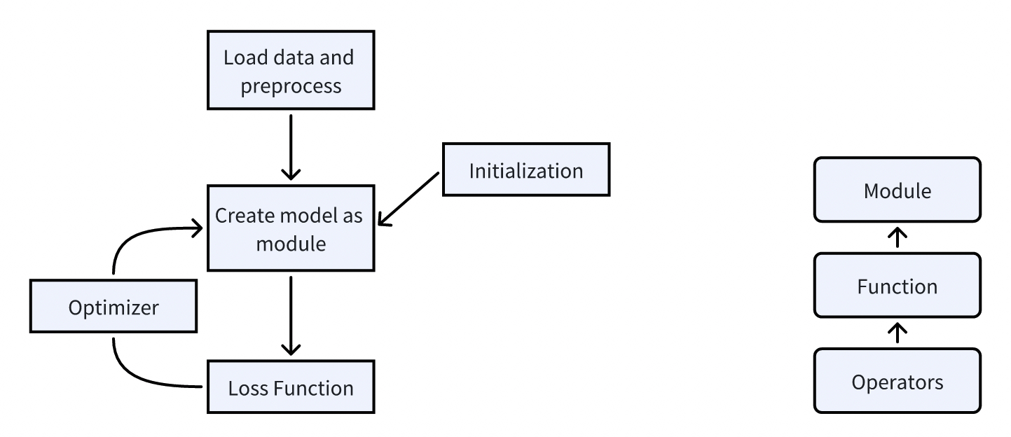
有了前述内容铺垫,Optimizer 相关代码就显得很简单了。其与 Module 模块通过 Module.parameters() 方法关联,获取模型的可学习参数。step() 方法根据不同的参数更新规则,进行参数更新。

5. Conclusion

  • Tensor
    • TensorData: shape & strides
  • Automatic Differentiation
    • Computation Graph: History & Context
    • Function
    • chain rule(implementation of backpropagate)
  • Module
    • Parameter
    • Module
  • Optimizer
    • step

LLM Systems Assignment 2: Minitorch Framework
https://arcsin2.cloud/posts/2026/10/2104219689/
作者
arcsin2
发布于
2026年10月5日
许可协议