Evaluate Dataset and Sample Difficulty
This article shares papers on evaluating datasets and sample difficulty, specifically:
- A Theory of Usable Information Under Computational Constraints
- Understanding Dataset Difficulty with \(\mathcal{V}\)-Usable Information
The main content comes from the sharing of the group meeting, the slides is right here.
1. Shannon Mutual Information
In probability theory and information theory, the mutual information (Mutual Information, MI) of two random variables measures the degree of mutual dependence between the two variables. Specifically, for two random variables, MI is the "information" (usually in bits) of one random variable that is reduced by knowing the other.
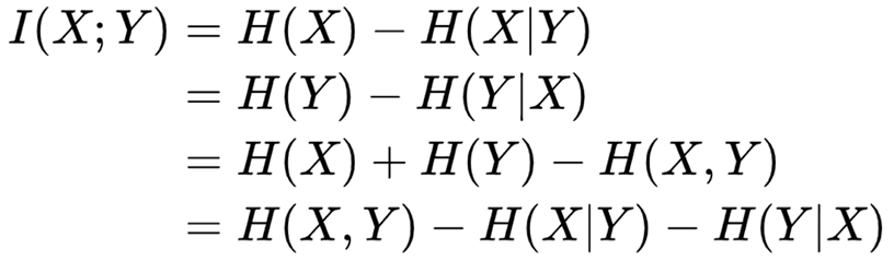
The mutual information of discrete random variables X and Y can be calculated as:

where p(x, y) is the joint probability mass function of X and Y, and p(x) and p(y) are the marginal probability mass functions of X and Y, respectively.
Mutual information can be equivalently expressed as:
However, in the context of machine learning, Shannon mutual information conflicts with some of our current empirical understanding, such as the example shown in the picture below:

Under Shannon's mutual information theory, the mutual information of the plaintext and the label is equal to the mutual information of the ciphertext and the label. However, for us humans, the label can be easily identified from the plaintext; it cannot be judged from the ciphertext. That is, as shown in the figure below:
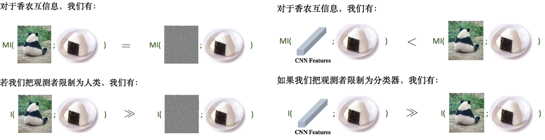
To resolve this conflict, the authors propose a new concept: considering mutual information under computational constraints.
2. Extended Definition of Shannon Mutual Information——\(\mathcal{V}\)-Information
First, the author introduces three concepts:
predictive family
Let \(\Omega=\{f: \mathcal{X} \cup\{\varnothing\} \rightarrow \mathcal{P}(\mathcal{Y})\}\). We say that \(\mathcal{V} \subseteq \Omega\) is a predictive family if it satisfies \[ \forall f \in \mathcal{V}, \forall P \in \operatorname{range}(f), \quad \exists f^{\prime} \in \mathcal{V}, \quad \text { s.t. } \quad \forall x \in \mathcal{X}, f^{\prime}[x]=P, f^{\prime}[\varnothing]=P \]
predictive conditional \(\mathcal{V}\)-entropy
Let \(X, Y\) be two random variables taking values in \(\mathcal{X} \times \mathcal{Y}\), and \(\mathcal{V}\) be a predictive family. Then the predictive conditional \(\mathcal{V}\)-entropy is defined as \[ \begin{aligned} H_{\mathcal{V}}(Y \mid X) & =\inf _{f \in \mathcal{V}} \mathbb{E}_{x, y \sim X, Y}[-\log f[x](y)] \\ H_{\mathcal{V}}(Y \mid \varnothing) & =\inf _{f \in \mathcal{V}} \mathbb{E}_{y \sim Y}[-\log f[\varnothing](y)] \end{aligned} \] We additionally call \(H_{\mathcal{V}}(Y \mid \varnothing)\) the \(\mathcal{V}\)-entropy, and also denote it as \(H_{\mathcal{V}}(Y)\) .
predictive conditional \(\mathcal{V}\)-information
Let \(X, Y\) be two random variables taking values in \(\mathcal{X} \times \mathcal{Y}\), and \(\mathcal{V}\) be a predictive family. The predictive \(\mathcal{V}\)-information from \(X\) to \(Y\) is defined as \[ I_{\mathcal{V}}(X \rightarrow Y)=H_{\mathcal{V}}(Y \mid \varnothing)-H_{\mathcal{V}}(Y \mid X) \]
\(\mathcal{V}\)-information has the following properties:
basic properties
Let \(Y\) and \(X\) be any random variables on \(\mathcal{Y}\) and \(\mathcal{X}\), and \(\mathcal{V}\) and \(\mathcal{U}\) be any predictive families, then we have
- Monotonicity: If \(\mathcal{V} \subseteq \mathcal{U}\), then \(H_{\mathcal{V}}(Y) \geq H_{\mathcal{U}}(Y), H_{\mathcal{V}}(Y \mid X) \geq H_{\mathcal{U}}(Y \mid X)\).
- Non-Negativity: \(I_{\mathcal{V}}(X \rightarrow Y) \geq 0\).
- Independence: If \(X\) is independent of \(Y, I_{\mathcal{V}}(X \rightarrow Y)=I_{\mathcal{V}}(Y \rightarrow X)=0\).
Data processing inequalities (different from Shannon mutual information)
- Shannon Mutual Information: Letting \(t: \mathcal{X} \rightarrow \mathcal{X}\) be any function, \(t(X)\) cannot have higher mutual information with \(Y\) than \(X: I(t(X) ; Y) \leq I(X ; Y)\).
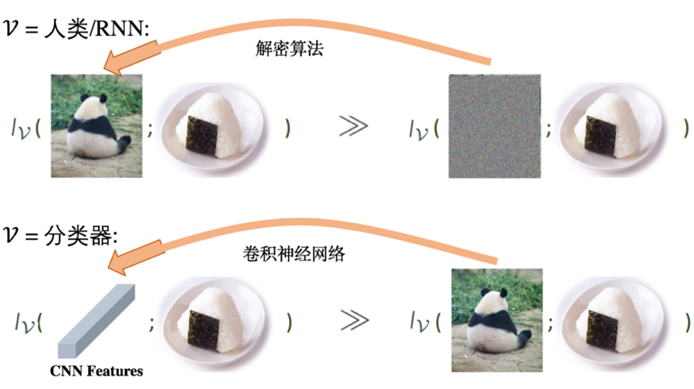
- \(\mathcal{V}\)-Information: Denoting \(t\) as the decryption algorithm and \(\mathcal{V}\) as a class of natural language processing functions, we have that: \(I_{\mathcal{V}}(t(X) \rightarrow Y)>I_{\mathcal{V}}(X \rightarrow Y) \approx 0\).
Asymmetry (different from Shannon mutual information)
If \(\mathcal{V}\) contains all polynomial-time computable functions, then \(I_{\mathcal{V}}(X \rightarrow h(X)) \gg I_{\mathcal{V}}(h(X) \rightarrow X)\) , where \(h: \mathcal{X} \rightarrow \mathcal{Y}\).
According to the nature of \(\mathcal{V}\)-information, we can reasonably explain the problems shown in the above example, thus:
The above is a strict definition of \(\mathcal{V}\)-Information, but in machine learning, we don't have a real distribution, but only a finite size data set sampled from the distribution. Next, the authors address how to estimate \(\mathcal{V}\)-Information on a finite-sized dataset:
Let \(X, Y\) be two random variables taking values in \(\mathcal{X}, \mathcal{Y}\) and \(\mathcal{D}=\left\{\left(x_i, y_i\right)\right\}_{i=1}^N \sim X, Y\) denotes the set of samples drawn from the joint distribution over \(\mathcal{X}\) and \(\mathcal{Y} . \mathcal{V}\) is a predictive family. The empirical \(\mathcal{V}\)-information (under \(\mathcal{D}\) ) is the following \(\mathcal{V}\)-information under the empirical distribution defined via \(\mathcal{D}\) : \[ \hat{I}_{\mathcal{V}}(X \rightarrow Y ; \mathcal{D})=\inf _{f \in \mathcal{V}} \frac{1}{|\mathcal{D}|} \sum_{y_i \in \mathcal{D}} \log \frac{1}{f[\varnothing]\left(y_i\right)}-\inf _{f \in \mathcal{V}} \frac{1}{|\mathcal{D}|} \sum_{x_i, y_i \in \mathcal{D}} \log \frac{1}{f\left[x_i\right]\left(y_i\right)} \] Then we have the following PAC bound over the empirical \(\mathcal{V}\)-information:
Assume \(\forall f \in \mathcal{V}, x \in \mathcal{X}, y \in \mathcal{Y}, \log f[x](y) \in[-B, B]\). Then for any \(\delta \in(0,0.5)\), with probability at least \(1-2 \delta\), we have: \[ \left|I_{\mathcal{V}}(X \rightarrow Y)-\hat{I}_{\mathcal{V}}(X \rightarrow Y ; \mathcal{D})\right| \leq 4 \mathfrak{R}_{|\mathcal{D}|}\left(\mathcal{G}_{\mathcal{V}}\right)+2 B \sqrt{\frac{2 \log \frac{1}{\delta}}{|\mathcal{D}|}} \] where we define the function family \(\mathcal{G}_{\mathcal{V}}=\{g \mid g(x, y)=\log f[x](y), f \in \mathcal{V}\}\), and \(\mathfrak{R}_N(\mathcal{G})\) denotes the Rademacher complexity of \(\mathcal{G}\) with sample number \(N\).
3. Evaluate Dataset and Sample Difficulty using \(\mathcal{V}\)-Information
Using the \(\mathcal{V}\)-Information tool introduced above and conducting experiments, some interesting phenomena can be found.
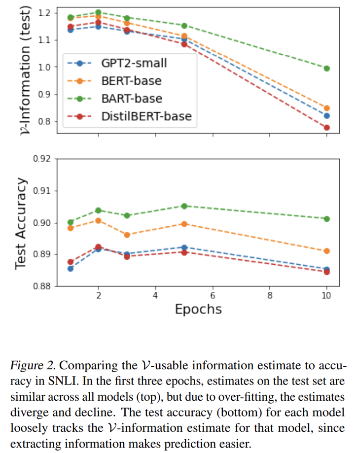
- The accuracy and \(\mathcal{V}\)-Usable Information of the large model are higher, because extracting more information makes recognition easier
- \(\mathcal{V}\)-Information is more sensitive to over-fitting compared to accuracy
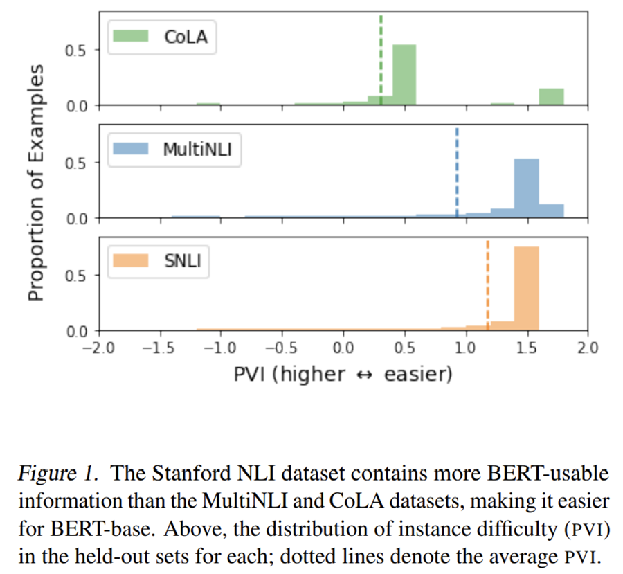
- Provides a way to measure the difficulty of different datasets
Then, a method for evaluating sample point \(\mathcal{V}\)-Information (Pointwise \(\mathcal{V}\)-Information, PVI) is introduced:
Given random variables \(X, Y\) and a predictive family \(\mathcal{V}\), the pointwise \(\mathcal{V}\)-information (PVI) of an instance \((x, y)\) is \[ \operatorname{PVI}(x \rightarrow y)=-\log _2 g[\varnothing](y)+\log _2 g^{\prime}[x](y) \] where \(g \in \mathcal{V}\) s.t. \(\mathbb{E}[-\log g[\varnothing](Y)]=H_{\mathcal{V}}(Y)\) and \(g^{\prime} \in \mathcal{V}\) s.t. \(\mathbb{E}\left[-\log g^{\prime}[X](Y)\right]=H_{\mathcal{V}}(Y \mid X)\).
PVI is to \(\mathcal{V}\)-information what PMI is to Shannon information: \[ \begin{aligned} I(X ; Y) & =\mathbb{E}_{x, y \sim P(X, Y)}[\operatorname{PMI}(x, y)] \\ I_{\mathcal{V}}(X \rightarrow Y) & =\mathbb{E}_{x, y \sim P(X, Y)}[\operatorname{PVI}(x \rightarrow y)] \end{aligned} \]
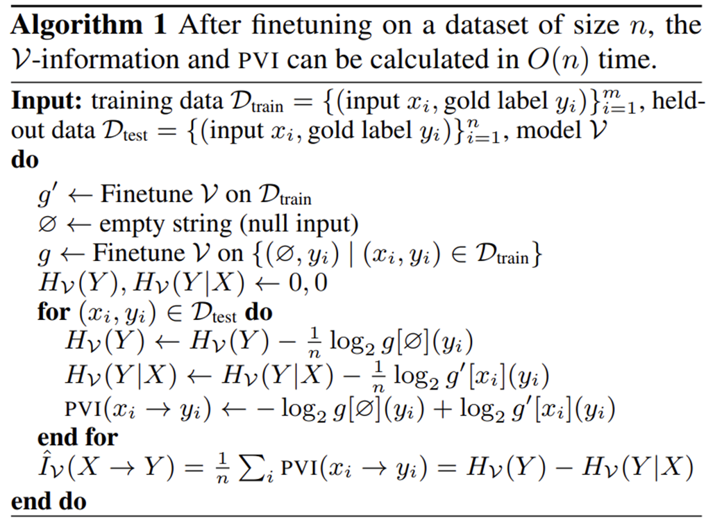
The complete algorithm flow is as follows:
Then, using PVI to experiment, we can also observe some interesting phenomena:
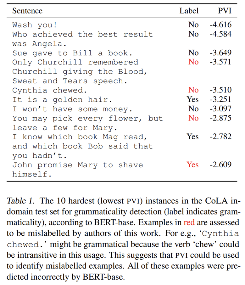
- There are many labeling errors in the sample with the lowest PVI
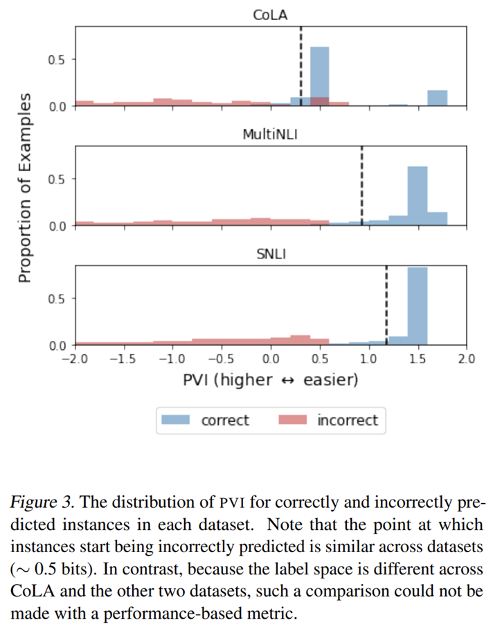
- The PVI threshold for the model to correctly classify samples is around 0.5
In addition, the original paper also showed some interesting experimental phenomena, which will not be repeated here, please refer to the original paper for details.