LLM Systems 16: Model Parallel Training
0.Recap
- Data Parallel via All Reduce
- Distributed Data Parallel Training
- gradient bucketing
- overlay backward and AllReduce communication
1. Model Parallel Training
Motivation: 模型规模呈指数增长,单个 GPU 的显存无法放置完整模型。模型并行就是将模型的计算(forward/backward/update)切分到多个训练进程。
Distributed layer-wise computation(PP)示意图:
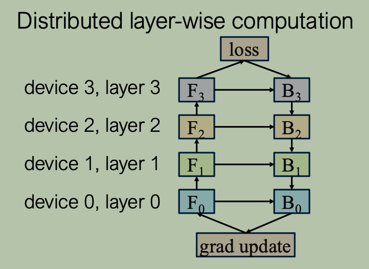
- 按层切分模型。
Distributed tensor computation(TP)示意图:
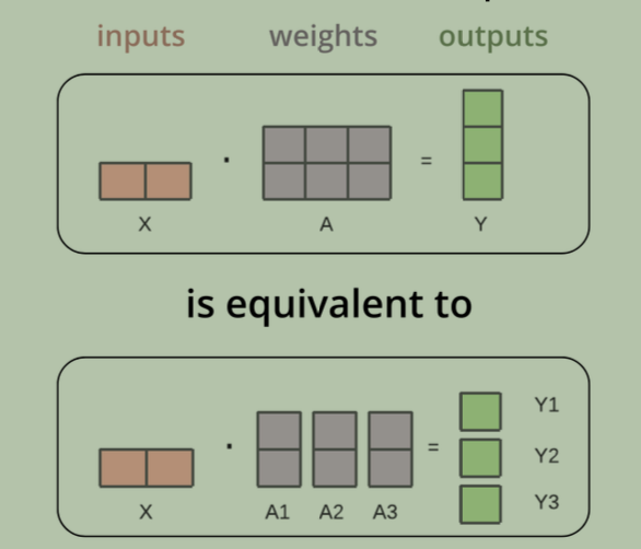
- 切分参与 GEMM 计算的模型权重。
2. Pipeline Parallelism
2.1 Naive Pipeline Parallel
实现:按层将模型切分放置在不同 GPU。
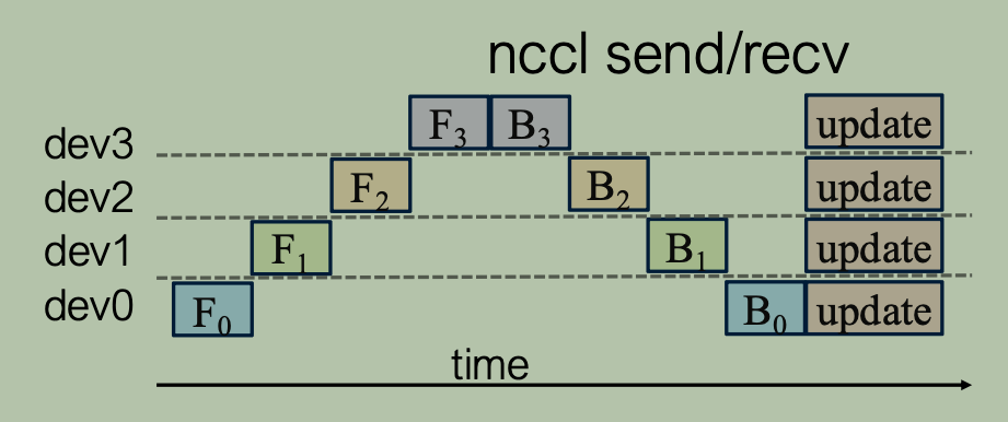
问题:在任意时刻,只有一个 GPU 进行计算,其他都空闲。如下图所示:
计算与显存分析:
下图来源:blog
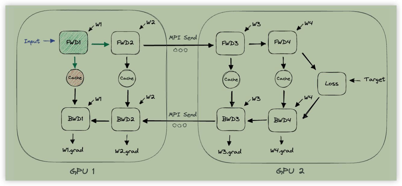
- 从上面左侧开始看,input 在 GPU 1 进行 forward,产生中间激活值需要缓存下来;
- 通过 P2P 通信 API,发生 GPU 1 forward 得到的激活值到 GPU 2;
- GPU 2 运行 forward,产生中间激活值;
- GPU 2 计算 loss 并进行 backward,自动求导引擎根据缓存激活值计算模型参数梯度;
- GPU 2 将 GPU 1 发送过来的激活值对应梯度通过 P2P 发送给 GPU 1;
- GPU 1 执行 backward,得到本 device 内参数梯度。
示例代码:
1 | |
朴素 PP 实现的问题:
- 低 GPU 利用率
- 任意时刻仅有一个 GPU 工作,其他空闲。
- 没有计算与通信的重叠
- 设备在通过网络(如 NCCL send/recv)向下一个设备传输中间激活值或梯度时,GPU 处于闲置状态,无法做到边计算边传输,通信开销无法被掩盖。
- 高显存需求
- 前向传播必须等整个 Mini-batch 完全通过所有设备后才能开启反向传播,靠前的设备(如第一张 GPU)必须长时间暂存整个 Batch 的所有中间激活值(Activations),直到反向传播计算结束。
2.2 Improving Pipeline Parallel: GPipe
2.2.1 Overview
- 核心思想:将输入的一个 batch (mini-batch)数据切分为多个小 batch(micro-batch),使用 micro-batches 进行流水线并行。
- batch 大小
- 决定因素:
- GPU memory 大小
- 每个样本 forward/backward 需要的显存大小
- batch 需要尽量大,以充分利用 GPU 显存;同时允许切分为更多 micro-batch 降低流水线 bubble。
- 决定因素:
- micro-batch 可以比 batch 小很多。
2.2.2 GPipe
- 相关符号及含义:
- 设模型有 \(L\) 层;
- 模型被切分为 \(K\) 个分区(即:device 数量);
- 每个 mini-batch 被切分为 \(M\) 个 micro-batch;
- mini-batch 大小为 \(N\) 。
- GPipe 整体流程:
- 切分为 micro-batch;
- 每个 micro-batch forward 完成后,立即将结果发送给下一个 device;
- 所有 micro-batches forward 完成后,再进行 backward;
- 在 backward 过程中,进行 forward 重计算,完成后立即将 micro-batches 梯度发送给上一个 device;
- 示意图如下:
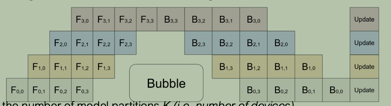
- 气泡比例:
- \(K\) 个 device 完成 \(M\) 个 micro-batches fwd/bwd 共需要时间面积为:\(K \times (M + K - 1) \times (t + 2t)\),其中 \(t\) 表示每个 device 完成一个 micro-batch forward 耗时;bwd 耗时认为是 fwd 两倍;\(M + K - 1\) 表示 \(K - 1\) 步用来建立完整流水线,\(M\) 步用来清空流水线(全部执行完成);
- 其中 bubble 面积为 \(K \times (K-1) \times (t + 2t)\) ;
- 整体 bubble 比例为:\(\frac{K \times (K-1) \times (t + 2t)}{K \times (M + K - 1) \times (t + 2t)} = \frac{K - 1}{M + K - 1}\) ;当 \(M > 4 \times K\) 时,气泡比例可忽略(\(M > 4K\) 时,实际气泡比例范围为:\((\frac{1}{9}, \frac{1}{5})\))。
- 通信开销:相邻 device 间需要进行 P2P 通信传输激活值。
- 激活值内存占用峰值:
- 朴素实现:\(O(N \times L)\)
- 单个 Micro-batch 在单张 GPU(含 \(\frac{L}{K}\) 层)上产生的所有激活值大小为:\(\text{单微批次激活值} = O\left(\frac{N}{M} \times \frac{L}{K}\right)\)
- 由于 GPipe 的调度特点是必须把所有 \(M\) 个微批次的前向传播全部做完,才能开始反向传播,因此显存里会同时积压 \(M\) 个微批次的所有激活值: \(\text{峰值显存} = M \times O\left(\frac{N}{M} \times \frac{L}{K}\right) = O\left(N \times \frac{L}{K}\right)\)
- 忽略设备常数 \(K\),即可简写为 \(O(N \times L)\)。
- gradient checkpoint:\(O(N + \frac{L}{K}
\times \frac{N}{M})\)
- 第一项 \(N\)(常驻显存,即 \(M\) 个微批次的边界激活值):
在前向传播过程中,每张 GPU 不再保存这 \(\frac{L}{K}\)
层内部所有的中间激活值,而只保存每个 Micro-batch
在设备输入/输出边界处的激活值(Boundary Checkpoints)。
- 单个 Micro-batch 的边界激活值大小为 \(O(\frac{N}{M})\);
- 全部 \(M\) 个 Micro-batch 的边界激活值总和为: \(M \times O\left(\frac{N}{M}\right) = O(N)\)
- 第二项(反向传播时的临时局部重算显存): 当反向传播计算到某个
Micro-batch 时,GPU 会利用该 Micro-batch
留下的边界激活值,临时重新计算该 Micro-batch 在单卡内 \(\frac{L}{K}\) 层的内部激活值。
- 同一时刻只需要重算 1 个 Micro-batch,所以这部分临时激活值开销仅为: \(O\left(\frac{N}{M} \times \frac{L}{K}\right)\) 。算完这个 Micro-batch 的梯度后,这部分临时激活值就会被立即释放,供下一个 Micro-batch 使用。
- 第一项 \(N\)(常驻显存,即 \(M\) 个微批次的边界激活值):
在前向传播过程中,每张 GPU 不再保存这 \(\frac{L}{K}\)
层内部所有的中间激活值,而只保存每个 Micro-batch
在设备输入/输出边界处的激活值(Boundary Checkpoints)。
- 朴素实现:\(O(N \times L)\)
Gradient Checkpointing
- 思想:
- forward:每个 device 只保存输入和输出激活值;
- backward:利用输入重新进行 forward 构建计算图,然后基于计算图进行 backward。
- 三种变体:\(n\) 表示模型层数
- 传统反向传播(Vanilla backprop):
- 激活值显存:\(O(n)\) —— 保存所有 \(n\) 层的中间激活值。
- 计算量:\(O(n)\) 。
- 极限省显存/完全重算(Memory poor backprop):
- 激活值显存:\(O(1)\) —— 几乎不保留中间激活值,只留输入。
- 计算量:\(O(n^2)\) —— 计算第 \(k\) 层梯度时,必须从第 1 层开始重新前向推演到第 \(k\) 层,导致计算量暴涨到二次方级。
- 梯度检查点(Gradient Checkpointing):
- 策略:每隔 \(\sqrt{n}\) 层保存一个 Checkpoint(检查点)。
- 激活值显存:\(O(\sqrt{n})\) —— 只需保留约 \(\sqrt{n}\) 个检查点处的激活值,实现亚线性(Sublinear)显存开销。
- 计算量:\(O(\sqrt{n} \times \sqrt{n}) = O(n)\) —— 反向传播时只在相邻检查点之间做局部重算,整体计算复杂度依然保持在 \(O(n)\)(选择适当 layer 做 gradient checkpoint 可以实现仅增加约 20%~30% 的前向重算耗时)。
- 传统反向传播(Vanilla backprop):
GPipe PP 缺点:
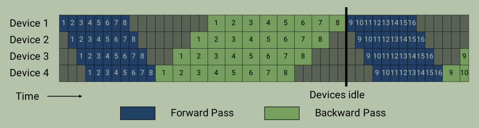
- 由于在全部 micro-batches forward 完成后才进行 backward,需要保存全部 micro-batches 的激活值,显存占用大。
Improving Pipeline Parallel with 1F1B flush
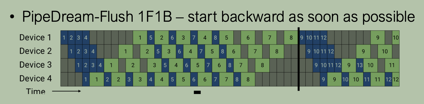
- 核心思想:尽早开始进行 backward 以减少中间激活值显存占用。
- 优点:减少激活值显存占用。
- GPipe 的激活值显存随着微批次总数 \(M\) 线性增长(\(O(M)\))。
- 1F1B 的激活值显存只与流水线深度/设备数 \(K\) 相关(\(O(K)\)),与微批次总数 \(M\) 无关。
- 在途(即已完成前向传播、但尚未完成反向传播)的 micro-batch 数量:最多为 4 个(假设一次反向传播耗时等于两次前向传播耗时,即 1B=2F),而在 GPipe 中则高达 8 个。
1F1B 实现:
流水线三个阶段:
- 预热期(Warmup):只做 Forward,把流水线灌满。
- 稳态期(Steady State):1F1B 交替(一前一后)。
- 收尾/冷却期(Cooldown / Drain):只做 Backward,清空流水线。
不同 GPU 在预热期和收尾期的步数不同。
Further Improving Pipeline Parallel by Chunking Model Layers and Interleaving Stages
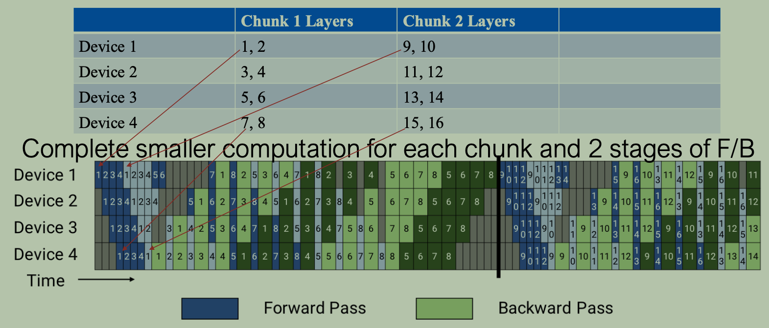
- 核心思想:把模型层切得更细,并在 GPU 之间“交错”分配
- 传统 1F1B(非交错式): 每张 GPU 只分配一段连续的模型层
- 交错式 1F1B(Slide 中的 Chunking 方案): 每张 GPU
不再只吃“一大块”连续层,而是分配多个较小且不连续的层切块(Chunks)。上图将
16 层切为了 2 个 Chunk(即切块数 \(v =
2\))
- Device 1 负责 Chunk 1(第 1, 2 层)和 Chunk 2(第 9, 10 层)
- ...
- 优点:气泡更少
- 气泡被切碎并压缩了 \(v\) 倍:
在流水线建立和清空的过程中,卡与卡之间等待的时间取决于单次计算的耗时。
- 传统 1F1B 单次计算需要跑 4 个层,等待时间较长。
- 交错式 1F1B 单次计算只需要跑 2 个层(耗时减半),因此首尾等待的气泡碎片时间也缩小到了原来的 \(\frac{1}{v}\)。
- 气泡占比:
- GPipe / 传统 1F1B:\(\text{Bubble 比例} \approx O\left(\frac{K - 1}{M + K - 1}\right)\) 。
- Interleaved 1F1B:\(\text{Bubble 比例} \approx O\left(\mathbf{\frac{1}{v}} \cdot \frac{K - 1}{M + K - 1}\right)\) 。
- 如果取 \(v = 2\),气泡占比直接折半;如果取 \(v = 4\),气泡占比可以缩小到原来的 \(\frac{1}{4}\),直接将原本 10%~15% 的算力浪费压缩到了 2%~5% 这种工程上几乎可以忽略不计的水平。
- 气泡被切碎并压缩了 \(v\) 倍:
在流水线建立和清空的过程中,卡与卡之间等待的时间取决于单次计算的耗时。
- 代价:
- P2P 通信频次与流量翻倍: 因为一个 Micro-batch
需要在设备链上完整跑 \(v\)
圈,网络通信(
send/recv)的触发次数和数据传输总量直接乘以了 \(v\)(上述示例图片中通信量翻了 2 倍)。 - 显存与调度逻辑更复杂: 每张 GPU 需要在显存中同时维护多个 Chunk 的激活值队列和状态转换,代码实现门槛大幅提高。
- P2P 通信频次与流量翻倍: 因为一个 Micro-batch
需要在设备链上完整跑 \(v\)
圈,网络通信(
PP 演进总结:
| 演进阶段 | 代表技术 | 核心机制 | 气泡占比 (Bubble) | 激活值显存峰值 |
|---|---|---|---|---|
| 第一代 | Naïve PP | 朴素纵向切分,无微批次 | 极大 (\(\frac{K-1}{K}\)) | \(O(\text{Batch Size})\) |
| 第二代 | GPipe | 微批次化 + 重算(全前向后全反向) | \(O\left(\frac{K-1}{M + K - 1}\right)\) | \(O(M)\)(随微批次线性暴涨) |
| 第三代 | 1F1B Flush | 预热后交替执行 1F/1B | \(O\left(\frac{K-1}{M + K - 1}\right)\) | \(O(K)\)(锁定上限,解绑 \(M\)) |
| 第四代 | Interleaved 1F1B | 模型切块交错(Chunking) | \(O\left(\frac{1}{v} \cdot \frac{K-1}{M + K - 1}\right)\) | \(O(K)\) |
GPipe Implementation:
代码来源:link
1 | |
Pipeline Parallelism in PyTorch
torch.distributed.pipelining 模块
- 两阶段
- build PipelineStage
- manually splitting the model
- splitting model automatically
- use PipelineSchedule for execution
- build PipelineStage
示例代码:
1 | |
3. Tensor Parallelism
3.1 Overview
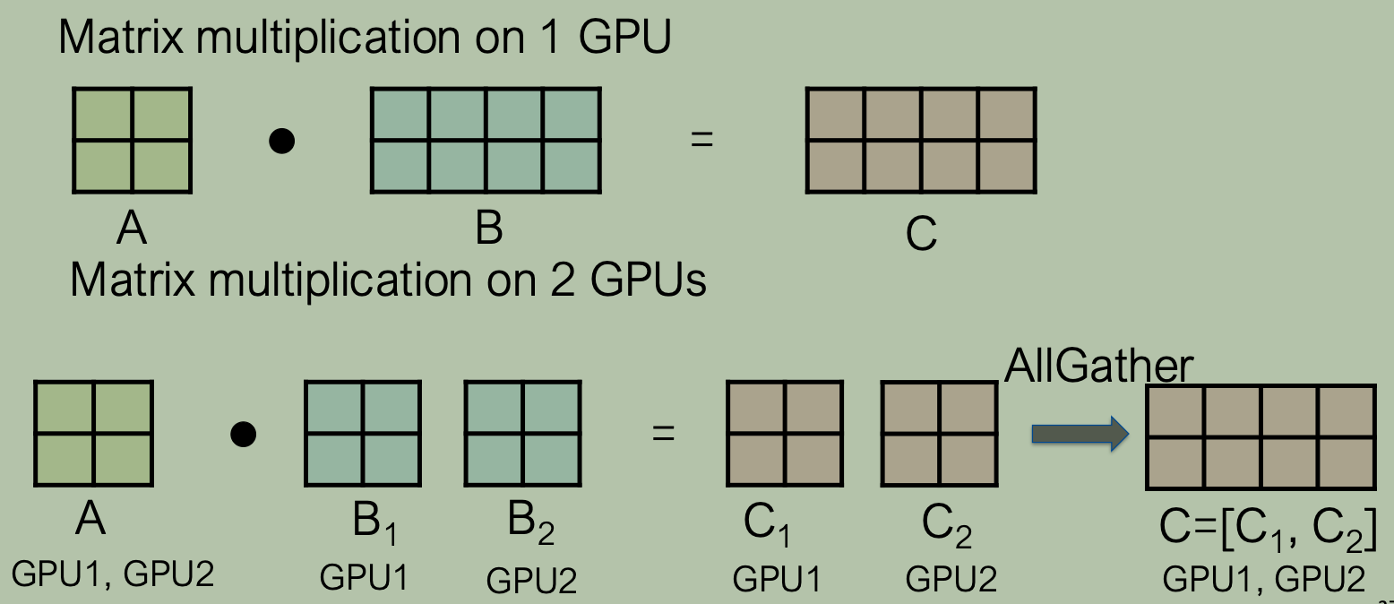
- 将参与 GEMM 的矩阵(模型参数)划分到多个 device 上,在各自 device 独立计算完成后,使用集合通信获取最终结果。
3.2 TP for FFN
考虑 FFN 输入为 \(X\);FFN 的第一个参数为 \(A\),第二个参数为 \(B\) 。
\(X\) 列切分 \(A\) 行切分:不可行
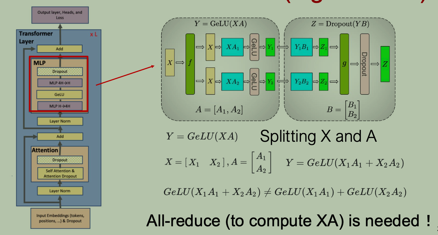
- 输入 \(X\) 按列切分,权重 \(A\) 按行切分方式如上图所示。
- 中间计算结果 \(Y\) 需要先经过 AllReduce 再进入 GeLU 激活函数,否则计算不等价:\(\text{GeLU}(X_1A_1 + X_2A_2) \neq \text{GeLU}(X_1A_1) + \text{GeLU}(X_2A_2)\)。
正确方式:\(A\) 列切分 \(B\) 行切分
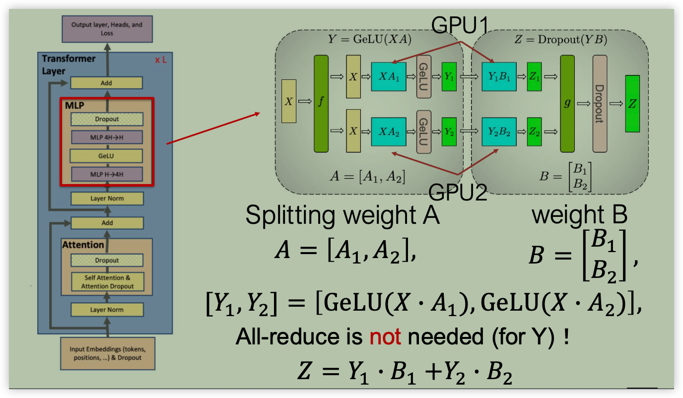
- 输入 \(X\) 不切分,重复输入两个 GPU;权重 \(A\) 按列切分;权重 \(B\) 按行切分;
- 中间计算结果 \(Y_{1,2} = XA_{1,2}\) 不需要通信,在各自 device 上独立经过 GeLU 激活函数即可;
- 最后计算结果 \(Z = Y_1B_1 + Y_2B_2\) 需要进行 AllReduce 求和。
3.3 TP for Self-Attention
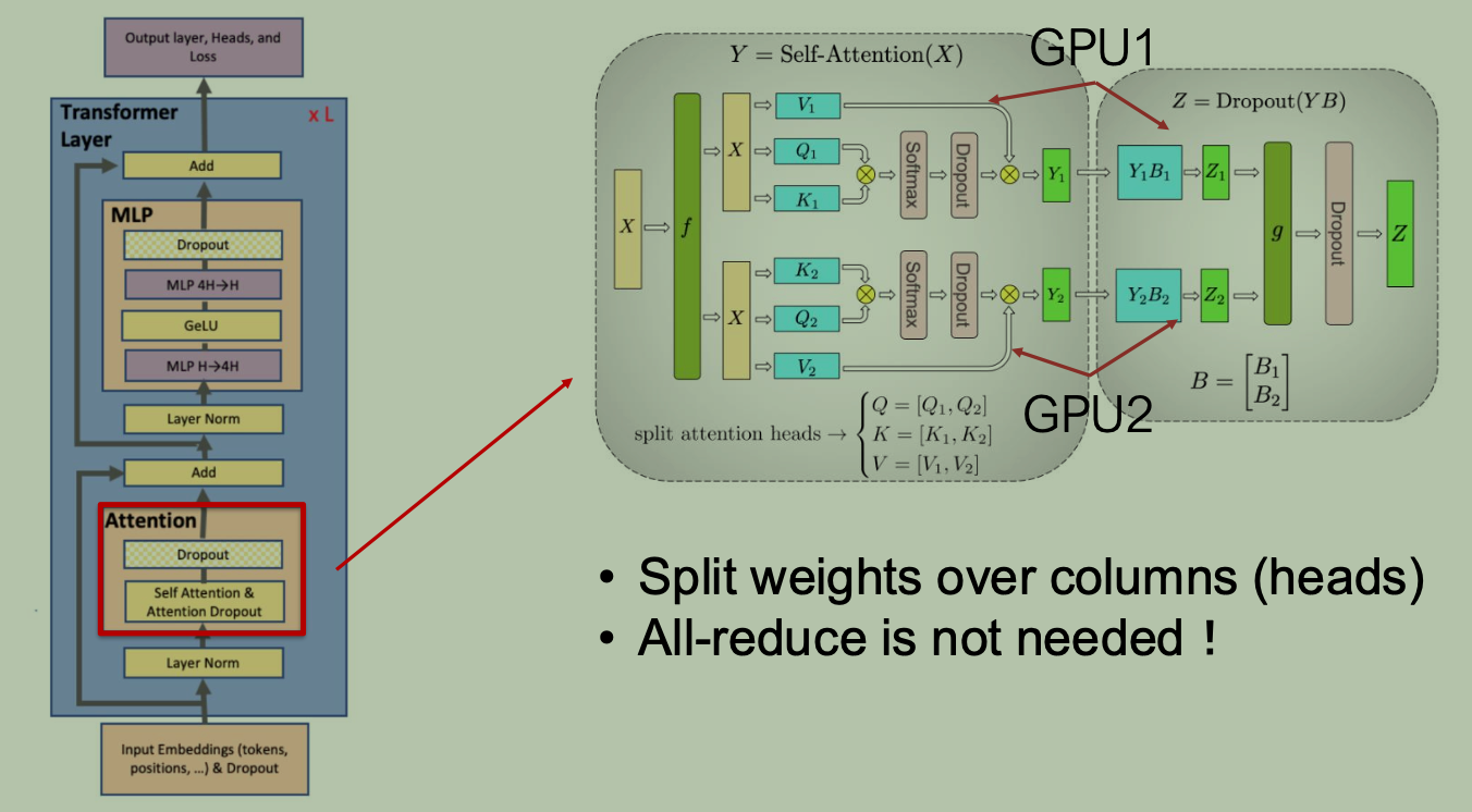
- MHA 回顾:
- 输入 tensor shape 为 \([B, S, H]\) ,分别表示 batch_size、序列长度、隐藏层维度。
- 模型参数包括:
- QKV 投影权重:\(Q\)、\(K\)、\(V\),shape 一般为 \([H, H]\)。设 MHA head 数量为 \(h\) ,则单个 head 对应权重维度为 \(\frac{H}{h}\) ,则 QKV 三个权重矩阵也可以看作 shape 为 \([H, h \cdot \frac{H}{h}]\) 。
- O 投影权重:\(O\) ,shape 一般为 \([H, H]\) 。
- forward 计算过程:
- 输入经过 QKV 投影权重,得到 QKV,shape 为 \([B, S, H]\) ;
- reshape/permute 输出,得到新 tensor shape 为 \([B, h, S, \frac{H}{h}]\) 。
- 计算 SelfAttention:\(\text{SelfAttention} = \text{Softmax}\left(\frac{QK^{T}}{\sqrt{d_k}} \right) V\) ,输出 shape 为:\([B, S, H]\)。
- 经过 \(O\) 投影权重,得到输出,shape 为 \([B, S, H]\) 。
- TP for MHA 切分及计算/通信过程:
- 切分原则:
- QKV 投影权重按 列 切分(相当于按 head 维度切分)
- 输出 O 投影权重按 行 切分
- 设有 \(P\) 个 device,则切分后每个
device 有 \(h_{local} = \frac{h}{P}\)
个 head,切分后 shape 情况:
- QKV 权重 shape 可以看作 \([H, \frac{h}{P} \cdot \frac{H}{h}]\) ;
- O 权重 shape 为 \([\frac{H}{P}, H]\) ;
- TP 切分后 forward 计算过程:
- 输入仍为全量 tensor,shape 为 \([B, S, H]\) ;
- 经过 local QKV 投影权重后,输出 tensor shape 为 \([B, S, \frac{H}{P}]\) ,等价于 \([B, S, \frac{h}{P} \cdot \frac{H}{h}]\) ;
- reshape/permute 后,QKV 输出 shape 可以看作 \([B, \frac{h}{P}, S, \frac{H}{h}]\) ;
- 计算 SelfAttention,输出 shape 为 \([B, S, \frac{H}{P}]\) ;
- 经过 local O 投影权重,得到输出 shape 为 \([B, S, H]\) ;
- TP group 进行 AllReduce 通信求和,得到最终输出结果。
- 切分原则:
3.4 TP for Embedding
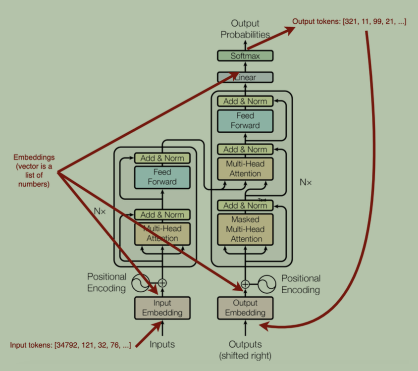
- Embedding 层
- 原始 shape (无 TP) 为 \([V, H]\) ,用来将每个 Embedding 映射为 \(H\) 维的 embedding。
- 按 行 切分,即词表中不同 token 对应的 embedding 被切分到不同 GPU 上;
- 切分后 forward 流程:
- 本地 local Embedding 查找,本地不存在的 token 返回全 0 embedding;
- 进行 AllReduce 通信求和,得到正确的 embeddings 输入。
- LM Head 层
- 原始 shape (无 TP)为 \([H, V]\) ,用来将隐藏层特征映射到词表 \(V\) 个 token。
- 按 列 切分,即每个 device 上切分后权重 shape 为 \([H, \frac{V}{P}]\);
- 切分后 forward 流程:
- 本地计算出自己负责的那部分词表 Logits,输出形状为 \([B, S, \frac{V}{P}]\) ;
- 朴素实现:通过 AllGather 获取全量 Logits,shape 为 \([B, S, V]\) ;
- 通信优化:通常会将输出与 Cross-Entropy Loss
进行算子融合,各卡只需跨卡规约局部最大值与指数和,避免传输海量
Logits,极大地削减通信开销。
- 第一次 AllReduce 获取全局 Logits 最大值 \(m\);
- 各卡基于全局最大值,计算本地 \(\sum{\exp{\left( x_{i}-m \right) } }\) ,然后进行第二次 AllReduce 通信获取全局和 \(S\);
- 只有包含目标 Token \(t\) 的那张 GPU 持有该 token 对应位置的 Logits,基于该 logit 计算出 loss。
- 通信量对比:原本需要传输形状为 \([B, S, V]\) 的庞大 Logits 张量,优化后压缩为了两个形状仅为 \([B, S]\) 的标量张量(\(m\) 与 \(S\)),通信体积直接缩小了数万倍(\(V/2\) 数量级)。
3.5 Other Layers in Tensor Parallel
- Layer normalization, dropout, residual connections
- Duplicate across GPUs
- 即:MHA/FFN 内部的残差连接计算,在每个 TP worker 内重复进行。
- TP Group 内有完全相同的 input tensor;
- local forward 完成后,进行 AllReduce 通信得到完全相同的 output tensor;
- TP Group 内所有 worker 都进行残差计算,得到 result = input +output,然后进入下一个模块计算;
- 然后所有 worker 独立计算可能的 LayerNorm/Dropout。
- 为了确保各卡独立做 Dropout 时算出的结果依然完全一致,TP Group 内部的
GPU 在执行这些重复层时,必须 共享相同的随机数种子(RNG
Seed) (Megatron-LM 内部通过
tensor_parallel.random模块专门维护了一套跨 TP 卡同步的 CUDA RNG State)。
- 为了确保各卡独立做 Dropout 时算出的结果依然完全一致,TP Group 内部的
GPU 在执行这些重复层时,必须 共享相同的随机数种子(RNG
Seed) (Megatron-LM 内部通过
- Each model parallel worker optimizes its own set of parameters
- 即:不同 worker 只负责 TP 切分后的 local 参数的梯度计算与参数更新。
3.6 Backward of Tensor Parallel
张量并行在反向传播中遵循严格的 正反向对偶性(Duality):
- 列并行(Column Parallel, 前向 \(f\) 算子):前向输入恒等/广播 \(\rightarrow\) 反向梯度做 All-Reduce (Sum)。
- 行并行(Row Parallel, 前向 \(g\) 算子):前向输出做 All-Reduce (Sum) \(\rightarrow\) 反向梯度恒等/广播(无通信)。
核心对偶规律总结:
| 正向行为 (Forward) | 语义 | 反向行为 (Backward) | 语义 |
|---|---|---|---|
| Broadcast / Replicate | 输入 \(X\) 被复制给多卡独立计算 | All-Reduce (Sum) | 梯度从多卡分支汇总累加 |
| All-Reduce (Sum) | 输出 \(Y\) 由多卡结果相加聚合 | Identity / Split | 梯度直接原样回传(无需通信) |
3.6.1 FFN (MLP) 模块的反向传播
- 升维层 \(W_{\text{in}}\)(列并行 Column
Parallel):
- 计算:各卡根据本地激活值计算本地权重的梯度 \(\frac{\partial \mathcal{L}}{\partial W_{\text{in}}^{(k)}}\)。
- 通信:由于前向传播时输入 \(X\) 是广播给所有卡的,因此向主干 \(X\) 传回梯度时,需要对各卡算出的 \(\frac{\partial \mathcal{L}}{\partial X^{(k)}}\) 执行 All-Reduce (Sum)。
- 降维层 \(W_{\text{out}}\)(行并行 Row
Parallel):
- 计算:上游回传的梯度 \(\frac{\partial \mathcal{L}}{\partial Z}\) 直接分发给各卡,本地计算 \(\frac{\partial \mathcal{L}}{\partial W_{\text{out}}^{(k)}}\) 和对中间激活值的梯度。
- 通信:无通信(前向的 All-Reduce 在反向变成了恒等分发)。
3.6.2 MHA (Self-Attention) 模块的反向传播
- QKV 投影层 \(W_{qkv}\)(列并行 Column
Parallel):
- 计算:本地各 Head 计算各自 \(Q, K, V\) 的梯度。
- 通信:将梯度传回输入的 Hidden State \(X\) 时,执行 All-Reduce (Sum)。
- Output 投影层 \(W_O\)(行并行 Row
Parallel):
- 计算:接收上游梯度,本地计算注意力 Context 的梯度。
- 通信:无通信。
3.6.3 Input Embedding 模块的反向传播(按 Vocab 行切分)
- 正向复习:各卡查表后做 All-Reduce (Sum) 得到全量特征。
- 反向计算:上游传回的梯度 \(\frac{\partial \mathcal{L}}{\partial Y}\) 直接广播给所有 GPU。
- 通信:无通信。每张 GPU 只需根据本地保存的 Token ID 索引,更新自己负责的那部分词表行的梯度即可。
3.6.4 LM Head + Fused Cross-Entropy 的反向传播(按 Vocab 列切分)
- 第一步:本地计算 Logits 梯度 Softmax + Cross-Entropy 的梯度公式: \[\frac{\partial \mathcal{L}}{\partial z_i} = p_i - y_i = \frac{e^{z_i - m}}{S} - \mathbf{1}(i = t)\] 因为正向传播时各卡已经拿到了全局的 \(m\) 和 \(S\),每张 GPU 可以在本地完全独立且精准地算出自己负责词片的 Logits 梯度 \(\frac{\partial \mathcal{L}}{\partial z^{(k)}}\),全程不需要跨卡交换 Logits。
- 第二步:反向传播至 Hidden State 本地 Logits 梯度与本地 LM Head 权重做矩阵乘法: \[\frac{\partial \mathcal{L}}{\partial X}_k = \frac{\partial \mathcal{L}}{\partial z^{(k)}} \cdot (W_{\text{head}}^{(k)})^T\]
- 第三步:通信 由于 LM Head 是列并行,各卡算出的 \(\frac{\partial \mathcal{L}}{\partial X^{(k)}}\) 需要通过 All-Reduce (Sum) 进行聚合,将完整的梯度传回 Transformer 最后一层的输出。
3.6.5 总结
| 模块 | 前向通信 (FWD) | 反向通信 (BWD) |
|---|---|---|
| Column Parallel (\(W_{qkv}, W_{\text{in}}, W_{\text{head}}\)) | 无 | All-Reduce (Sum) |
| Row Parallel (\(W_O, W_{\text{out}}\)) | All-Reduce (Sum) | 无 |
| Input Embedding (Vocab 行切) | All-Reduce (Sum) | 无 |
| Fused Cross-Entropy | All-Reduce (Max) + All-Reduce (Sum)(标量) | 无(利用 FWD 缓存标量直接本地算) |
3.7 Put All Together: Example
3.7.1 模型结构与切分配置 (Setup)
假设模型配置如下:
- TP 组:GPU 0, GPU 1 (\(P = 2\))
- 模型结构:
- Input Embedding:按词表 \(V\) 行切分(\(E_0, E_1\))
- Block 1:\(MHA_1\) (\(W_{qkv1}\) 切列, \(W_{O1}\) 切行) + \(FFN_1\) (\(W_{in1}\) 切列, \(W_{out1}\) 切行)
- Block 2:\(MHA_2\) (\(W_{qkv2}\) 切列, \(W_{O2}\) 切行) + \(FFN_2\) (\(W_{in2}\) 切列, \(W_{out2}\) 切行)
- LM Head + Fused CE:\(W_{\text{head}}\) 按词表 \(V\) 列切分(\(W_{\text{head}}^{(0)}, W_{\text{head}}^{(1)}\))
3.7.2 前向传播流程 (Forward Pass)
Step 0: Input Embedding (行切分)
- GPU 0 / GPU 1 拿着相同的 Input Token IDs 在各自本地的词表切片 \(E_0, E_1\) 中查表。
- 【通信 1 - FWD】:两卡执行 All-Reduce (Sum),获得完全相同的隐藏状态 \(X_0\)。
Step 1: Transformer Block 1
- \(MHA_1\):
- 两卡用 \(X_0\) 分别乘以本地列切片的 \(W_{qkv1}^{(k)}\),做本地 Attention 计算(无通信)。
- 经过本地行切片 \(W_{O1}^{(k)}\) 得到局部 Output。
- 【通信 2 - FWD】:两卡执行 All-Reduce (Sum),加和得到 \(MHA_1\) 的完整输出 \(A_1\)。
- 各卡本地计算残差:\(X_1 = X_0 + A_1\)。
- \(FFN_1\):
- 两卡用 \(X_1\) 乘以本地列切片 \(W_{in1}^{(k)}\) \(\rightarrow\) GeLU(无通信)。
- 乘以本地行切片 \(W_{out1}^{(k)}\) 得到局部 Output。
- 【通信 3 - FWD】:两卡执行 All-Reduce (Sum),得到 \(FFN_1\) 完整输出 \(F_1\)。
- 各卡本地计算残差:\(X_2 = X_1 + F_1\)。
Step 2: Transformer Block 2
- \(MHA_2\):
- 本地列切片 \(W_{qkv2}^{(k)}\) 计算,再过行切片 \(W_{O2}^{(k)}\)。
- 【通信 4 - FWD】:两卡执行 All-Reduce (Sum),得到 \(A_2\)。
- 本地残差:\(X_3 = X_2 + A_2\)。
- \(FFN_2\):
- 本地列切片 \(W_{in2}^{(k)}\) 计算,再过行切片 \(W_{out2}^{(k)}\)。
- 【通信 5 - FWD】:两卡执行 All-Reduce (Sum),得到 \(F_2\)。
- 本地残差:\(X_4 = X_3 + F_2\)。
Step 3: LM Head + Fused Cross-Entropy (列切分)
- 各卡用最终隐藏状态 \(X_4\) 乘以本地列切片 \(W_{\text{head}}^{(k)}\),算出局部 Logits 切片 \(z^{(k)}\)。
- 【通信 6 - FWD】:两卡算本地 Max,执行 All-Reduce (Max),得到全局 \(m = \max(z)\)。
- 【通信 7 - FWD】:两卡算本地 \(\sum e^{z^{(k)}-m}\),执行 All-Reduce (Sum),得到全局 \(S = \sum e^{z-m}\)。
- 本地根据 \(m\) 和 \(S\) 直接算出 Loss \(\mathcal{L}\)。
3.7.3 反向传播流程 (Backward Pass)
Step 3: LM Head + Fused Cross-Entropy (反向)
- 本地梯度:各卡利用 FWD 缓存的全局 \(m\) 和 \(S\),直接在本地算出 Logits 梯度 \(dz^{(k)} = p^{(k)} - y^{(k)}\)(无通信)。
- 反向投影:本地计算对隐藏状态的梯度 \(dX_4^{(k)} = dz^{(k)} \cdot (W_{\text{head}}^{(k)})^T\)。
- 【通信 1 - BWD】:因为 \(W_{\text{head}}\) 前向是列并行,反向传回主干 \(X_4\) 时执行 All-Reduce (Sum),得到完整的梯度 \(dX_4\)。
Step 2: Transformer Block 2 (反向)
- \(FFN_2\) 反向:
- 梯度 \(dX_4\) 沿着残差分支流向 \(FFN_2\) 的输出端 \(dF_2 = dX_4\)。
- 经过行切片 \(W_{out2}^{(k)}\) 反向传播(行并行反向无通信),得到中间梯度。
- 经过列切片 \(W_{in2}^{(k)}\) 反向传播,算出局部输入梯度 \(dX_3^{(k)}\)。
- 【通信 2 - BWD】:列并行反向传给主干,执行 All-Reduce (Sum),得到累加后的梯度 \(dX_3\)(包含残差分支)。
- \(MHA_2\) 反向:
- 梯度 \(dX_3\) 流向 \(MHA_2\) 输出端 \(dA_2 = dX_3\)。
- 经过行切片 \(W_{O2}^{(k)}\) 反向(无通信)。
- 经过列切片 \(W_{qkv2}^{(k)}\) 反向,算出局部输入梯度 \(dX_2^{(k)}\)。
- 【通信 3 - BWD】:执行 All-Reduce (Sum),得到累加后的梯度 \(dX_2\)。
Step 1: Transformer Block 1 (反向)
- \(FFN_1\) 反向:
- 行切片 \(W_{out1}^{(k)}\) 反向(无通信) \(\rightarrow\) 列切片 \(W_{in1}^{(k)}\) 反向。
- 【通信 4 - BWD】:执行 All-Reduce (Sum),得到 \(dX_1\)。
- \(MHA_1\) 反向:
- 行切片 \(W_{O1}^{(k)}\) 反向(无通信) \(\rightarrow\) 列切片 \(W_{qkv1}^{(k)}\) 反向。
- 【通信 5 - BWD】:执行 All-Reduce (Sum),得到 \(dX_0\)。
Step 0: Input Embedding (反向)
- 梯度 \(dX_0\) 回传至 Input Embedding 层。
- 每张 GPU 根据本地保存的 Token IDs,用 \(dX_0\) 直接更新各自本地行切片 \(E_k\) 的梯度(无通信)。
3.7.4 通信汇总表 (Communication Summary)
对于这个 2 层的 Transformer 模型,全流程通信次数统计如下:
| 阶段 | 通信算子及次数 | 详细分布 |
|---|---|---|
| 前向传播 (FWD) | 7 次 | 1 次 Embedding (All-Reduce Sum) + 4 次 Block 1&2 MHA/FFN ( All-Reduce Sum) + 2 次 Fused CE ( All-Reduce Max + All-Reduce Sum 标量) |
| 反向传播 (BWD) | 5 次 | 1 次 LM Head (All-Reduce Sum) + 4 次 Block 1&2 MHA/FFN ( All-Reduce Sum) (Embedding 与 Fused CE 均无通信) |
3.8 Example Code: FFN TP
1 | |
_CopyToModelParallelRegion:- 在 ColumnParallelLinear 输入端使用。FWD
不做通信;在 BWD 阶段时,反向传播回传给主干
(X) 的梯度会自动触发
All-Reduce (Sum)。
- 在 ColumnParallelLinear 输入端使用。FWD
不做通信;在 BWD 阶段时,反向传播回传给主干
(X) 的梯度会自动触发
_ReduceFromModelParallelRegion:- 在 RowParallelLinear 输出端使用。FWD 执行 1 次
All-Reduce (Sum)把各卡算出的局部 (Z_k) 加起来;在 BWD 阶段时为恒等分发(无通信)。
- 在 RowParallelLinear 输出端使用。FWD 执行 1 次
- Bias 处理:
- ColumnParallel 的 Bias 按列切分,直接加在本地输出上;
- RowParallel 的 Bias 属于全局 (H) 维度,必须放在
All-Reduce聚合之后再相加,避免重复累加。
4. Combination of PP/TP/DP
4.1 Combination of PP & TP
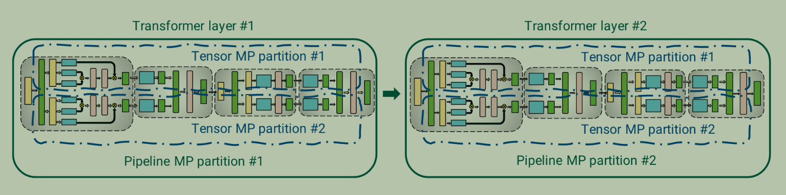
- PP=2, TP=2
- 2 层,每层 TP 划分到两个 GPU;不同层之间 PP 连接
- 通信分析:
- GPU 与 TP/PP Group 划分:
- TP Groups:
{GPU 0, GPU 1}(Stage 1)、{GPU 2, GPU 3}(Stage 2) - PP Groups:
PP Group 0(TP Rank 0 组):{GPU 0, GPU 2}PP Group 1(TP Rank 1 组):{GPU 1, GPU 3}
- TP Groups:
- TP Group 内做 AllReduce 通信;
- PP Group 内(TP Group 间相同 TP rank 的)做 P2P 通信;
- GPU 与 TP/PP Group 划分:
- PP/TP 设置取决于模型结构与服务器配置
- TP 设置一般最大是每个 GPU server 的 GPU 数,因为 TP 对通信带宽要求更高,即:TP for in-node parallel computing。
4.2 Model Parallel + Data Parallel
- 同时使用模型并行与数据并行:一个模型进行训练需要 \(M = t \times p\) 个 GPU 。此时可以利用 DP 继续扩展 GPU 数量提升训练吞吐。
工业界大模型训练的最佳并行组合优先级为:
- 单节点内(In-node):优先使用 张量并行(TP),充分利用节点内极高带宽的 NVLink/NVSwitch。
- 跨节点模型切分(Inter-node MP):当节点内显存装不下时,引入 流水线并行(PP) 将模型按层切分到多节点,直到显存完全够用。
- 跨节点算力扩展(Inter-node DP):一旦模型能正常跑起来不 OOM,剩余的所有 GPU 节点全部用于 数据并行(DP),以提升吞吐量与训练速度。
5. Conclusion
- Pipeline Parallelism
- split by layers (horizonal split)
- eliminate the bubbles (idle)
- interleaving forward/backward
- Tensor Parallelism
- split the matrix computation over multiple GPUs
- usually within a single node